


- Download PDF
- |
- Download Citation
- |
- Email a Colleague
- |
- Share:
-
- Tweet
-
Journal of Radiology and Imaging
Volume 4, Issue 2, February 2020, Pages 7–16
Original researchOpen Access
An analytical method for 3-dimensional calculation of the contaminant X-ray dose in water caused by clinical electron-beam irradiation
-
Akira Iwasaki1,*
 , Shingo Terashima2, Shigenobu Kimura3, Kohji Sutoh3, Kazuo Kamimura3, Yoichiro Hosokawa2 and
Masanori Miyazawa4
, Shingo Terashima2, Shigenobu Kimura3, Kohji Sutoh3, Kazuo Kamimura3, Yoichiro Hosokawa2 and
Masanori Miyazawa4
*Corresponding authors: Akira Iwasaki, 2-3-24 Shimizu, Hirosaki, Aomori 036-8254, Japan. Tel.: +172-33-2480; Email: fmcch384@ybb.ne.jp or fmcch384@gmail.com; and Shingo Terashima, Graduate School of Health Sciences, Hirosaki University, 66-1 Hon-cho, Hirosaki, Aomori 036-8564, Japan. Tel.: +81-172-39-5525; Email: s-tera@hirosaki-u.ac.jp
Received 20 November 2019 Revised 14 January 2020 Accepted 24 January 2020 Published 31 January 2020
DOI: http://dx.doi.org/10.14312/2399-8172.2020-2
Copyright: © 2020 Iwasaki A, et al. Published by NobleResearch Publishers. This is an open-access article distributed under the terms of the Creative Commons Attribution License, which permits unrestricted use, distribution and reproduction in any medium, provided the original author and source are credited.
AbstractTop
Purposes: In this paper, an analytical method for 3-dimensional (3D) calculation of the contaminant X-ray dose in water caused by clinical electron-beam irradiation is proposed in light of the two groups of Monte Carlo (MC) datasets reported by Wieslander and Knöös (2006). Methods: The dose calculation was performed based on Clarkson’s sector method. We used a plane called the isocenter plane, which is set perpendicular to the beam axis, containing the isocenter on it. On the isocenter plane, we defined the applicator field formed by an electron applicator and the cerrobend area field formed by a cerrobend insert if any, as well as other physical terms that are important for the dose calculations. The original sector method was modified to consider the following terms: (a) the vague beam-field margins formed by the dual-foil system; (b) the in-air dose distribution of the contaminant X-ray beam; (c) the X-ray spectrum change between the contaminant X-ray PDD datasets and the published radiotherapy X-ray PDD datasets; and (d) the contaminant X-ray attenuation for the cerrobent insert, if any. Results and conclusions: By comparing the calculated datasets of depth dose (DD) and off-axis dose (OAD) with the MC results for electron beams of E=6, 12, and 18 MeV, it can be concluded that the analytical calculation method is of practical use for various irradiation conditions. In particular, it should be noted that the analytical method can give almost the same calculation results as the MC-based dose calculation algorithm used in a commercial treatment planning system (TPS).
Keywords: clinical electron-beams; contaminant X-ray dose; electron applicator; linear accelerator; scattering foil; Clarkson’s sector method
Research highlightsTop
Based on Clarkson’s sector method, we developed an analytical method for calculation of the contaminant X-ray dose in water caused by clinical electron-beam irradiation. The analytical method was constructed by considering the following terms: (a) the vague beam-field margins formed by the dual-foil system; (b) the in-air dose distribution of the contaminant X-ray beam; (c) the X-ray spectrum change between the contaminant X-ray PDD datasets and the published radiotherapy X-ray PDD datasets; and (d) the contaminant X-ray attenuation for the cerrobent insert, if any. The dose calculation was performed in light of the two groups of Monte Carlo (MC) datasets reported by Wieslander and Knöös (2006). We conclude that the analytical method can achieve accurate dose calculations, even for beams with cerrobent inserts.
IntroductionTop
Khan [1] describes the physical outline of high-energy electrons used in radiation therapy as follows: The most useful energy for electrons is 6 to 20 MeV. At these energies, the electron beams can be used to treat superficial tumors (less than 5 cm deep) with a characteristically sharp drop-off in dose beyond the tumor. The principal applications are (a) the treatment of skin and lip cancers, (b) chest wall irradiation for breast cancer, (c) administering boost dose to nodes, and (d) the treatment of head and neck cancers. Although many of these sites can be treated with superficial X-rays, brachytherapy, or tangential photon beams, the electron-beam irradiation offers distinct advantages in terms of dose uniformity in the target volume and in minimizing the dose to deeper tissues.
Acceptable field flatness and symmetry are obtained [1] with a proper design of beam scatterers and beam defining collimators. Accelerators with magnetically scanned beam do not require scattering foils. Others use one or more scattering foils, usually made up of lead, to widen the beam as well as give a uniform dose distribution across the treatment field. In recent years, linear accelerators with scattering foil, having photon and multi-energy electron-beam capabilities, have become increasingly available for clinical use. Regarding the unnecessary contaminant X-ray dose caused when electron-beam irradiation occurs using linear accelerators, Mahdavi et al. [2] summarize as follows: (a) the contaminant X-ray dose provides a small dose to the patient; (b) the major part of the contaminant X-rays is produced by the accelerator exit window tube, monitor chamber, scattering foil, upper and lower pairs of collimator jaws, and electron applicator; (c) the scattering foil is the main source [3] and causes X-ray contamination, especially at high energies [4]; (d) the atomic number and thickness of the scattering foil have a mass effect on the X-ray contamination [5]; and (e) recently, a dual-foil system has been used, which is composed of the first and second foils (Figure 1), and this foil system can generate broader electron beams with less X-ray contamination, especially at high energies.
It should be emphasized that the contaminant X-ray dose is relatively small by comparison with the maximum electron-beam dose on the isocenter axis; however, the contaminant X-ray dose should not generally be ignored for accurate dose evaluation. It seems that nobody has reported how to calculate the 3D contaminant X-ray dose analytically. The analytical dealing is important for understanding the process of producing the contaminant X-ray dose. Monte Carlo (MC) methods are today widely used in many electron-beam therapy applications because of the complexity of photon and electron transport. Wieslander and Knöös [6, 7] proposed implementation of a virtual linear accelerator (based on MC simulations) into a commercial treatment planning system (TPS) to verify the TPS. The characterization set for the TPS includes depth doses, profiles, and output factors. The authors also emphasize that problems associated with conventional measurements can be avoided and properties that are considered unmeasurable can be studied because the MC method can divide the dose into the separate doses yielded by direct electrons, indirect electrons, and contaminant X-rays. They summarized two groups of MC dose datasets [7] for electron-beams of energies of 6, 12, and 18 MeV under a series of electron applicators using an Elekta Precise linear accelerator. Here, we refer to the datasets of interest as “the W-K MC dose datasets” or “the W-K MC dose work.” These datasets were yielded using a common virtual accelerator for two MC simulation techniques: one is the standard simulation, and the other is the simulation used in a commercial TPS.
The present paper will propose an analytical method for calculation of the contaminant X-ray dose in water in light of the two groups of W-K MC dose datasets. The analytical method is based on Clarkson’s sector method [1], but considers the vague beam-field margins caused by using the dual-foil system.
Materials and methodsTop
Symbols and units
This paper uses the following units: the lengths are expressed in cm; the areas are expressed in cm2; the angles are expressed in radian; and the doses are expressed in Gy. It should also be noted that some other physical quantities are dimensionless.
Theoretical background
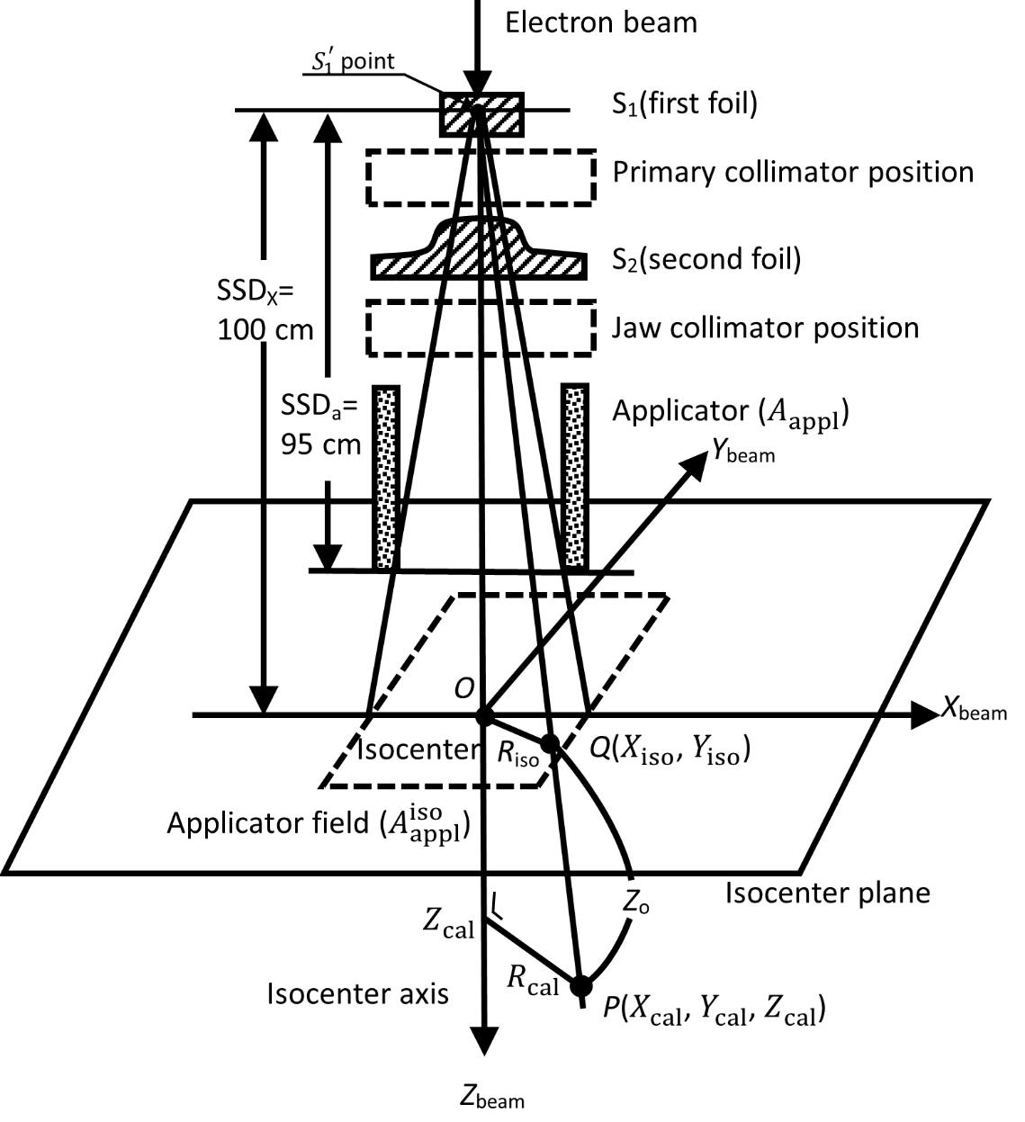
Figure 1 is redrawn with reference to the text-book by Khan [1], showing a typical arrangement for electron-beam irradiation using the dual-foil system. The first foil (S1) widens the narrow electron beam by multiple scattering, and the second foil (S2) is designed to make the widened electron beam uniform in cross-section (these two foils are installed in the treatment head of the accelerator). The thickness of the S2 foil is differentially varied across the beam to produce the desired degree of beam widening and flattening. The beam-defining collimators are designed to provide a variety of field sizes and to maintain or improve the cross-sectional flatness of the beam. Basically, the beam-defining collimators provide a primary collimation close to the S1 foil that defines the maximum field size and a secondary collimation close to the patient (or the isocenter plane) to define the treatment field. The secondary collimation is performed using the X-ray collimator jaws and a series of electron applicators. It should be noted that the X-ray collimator jaws are usually opened to a size larger than the electron applicator opening (in rectangles). Because the X-ray collimator jaws give rise to extensive electron scattering, they are interlocked with the individual electron applicators to open automatically to a fixed predetermined size.
It should be stressed that the contaminant X-rays are primarily generated in the S1 foil, and the amount of the contaminant X-rays varies in general with the field size (or electron applicator opening). We use a simple assumption here that the contaminant X-rays are all produced at a point ( ) on the isocenter axis within the S1 foil, as shown in Figure 1 (this paper does not directly refer to the dose caused by the bremsstrahlung produced by the electrons running through the phantom). This diagram also shows a geometrical arrangement for the contaminant X-ray dose calculation using a semi-infinite water phantom whose surface coincides with the isocenter plane on which the isocenter (O) is situated. Let SSDX be the distance between the point and the isocenter (O), and let SSDa be the distance between the point and the beam exit side of the electron applicator. Furthermore, we set orthogonal coordinates of Xbeam, Ybeam, and Zbeam whose origin is placed at the isocenter (O), where the Xbeam and Ybeam axes are set on the isocenter plane, and the Zbeam axis is drawn down from the isocenter (O), coinciding with the isocenter axis (or the beam axis). Let the dose calculation be performed at an arbitrary point P(Xcal, Ycal, Zcal) within the water phantom, definined as
 (Eq. 1)
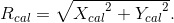
Let the intersection of the line P and the isocenter plane be denoted Q(Xiso, Yiso) (P is one of the fanlines radiating from point ), defined as
 (Eq. 2)
Let Z0 be the water length of point P, measured from point Q(Xiso, Yiso) along the line P; then, we have
 (Eq. 3)
The present analytical method is constructed for calculation of the contaminant X-ray dose at point Q(Xiso, Yiso), which is based on Clarkson’s sector method [1], described as follows:
(a) Let E be the electron-beam energy (MeV). Here, it is assumed that the contaminant X-rays are all produced in the S1 foil by the E-MeV electrons coming out from the accelerator with an acceleration voltage of E (MV).
(b) We utilize published radiotherapy X-ray percentage depth dose (PDD) datasets for a source-surface distance (SSD) of 100 cm. Here, we use Zmax(E) as the depth of maximum dose, letting it be simply determined only by E(MV) around a field of 10×10 cm2.
(c) Let the contaminant X-ray dose calculation be performed in a semi-infinite water phantom placed at an SSD of 100 cm, assuming that the dose is under lateral electron equilibrium and that the contaminant X-ray beam intensity in air at SSD=100 cm is the in-air dose measured in a small mass of water under forward and lateral electron equilibrium.
(d) We use electron applicators forming rectangular beam fields (the dose calculations are performed by neglecting the fine structures of the applicators). Let 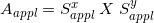 be denoted as the beam field measured at the beam exit side of the electron applicator. Let
  be the beam field measured on the isocenter plane. As the field is shaped by the fanlines emanating from the point, the field can be described as
 (Eq. 4)
Conversely, we let  be the field size that the X-ray collimator jaws form on the isocenter plane. As described earlier, we have >. Therefore, it can be seen that the more accurate intensity of the contaminant X-ray beam should be evaluated [1] based on . This paper uses cerrobend inserts only within the electron applicator field (this is because the W-K MC dose datasets are all collected under such irradiation conditions). It should be noted that the W-K MC dose datasets are produced with SSDX=100 cm and SSDa=95 cm using
  =10×10,14×14, and 20×20 cm2 (these dimensions are defined at SSD=SSDa [7]) for E = 6, 12, and 18 MeV.
(e) Let  (, E ) be the relative in-air dose intensity (refer to (c)) of the contaminant X-ray beam of E at the isocenter (O) when using an electron applicator of with no cerrobend insert.
(f) Let  (
( ) be the attenuation factor for the contaminant X-ray beam of E for a cerrobend insert with a thickness of
  (≤1, setting (=0, E )=1).
(g) For calculation of the relative in-air dose for the contaminant X-ray beam of E with no beam shielding insert for a point of Q(Xiso, Yiso) on the isocenter plane, we utilize the following function:
 (Eq. 5)
The relative in-air dose calculation for any combination of and E is then simply performed symmetrically with respect to the isocenter (O) on the isocenter plane, taking 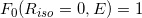 . Because the jaw field () determined by the electron applicator field () forms a perfect or approximate square field, the above F0 function is practically reasonable for use.
(h) The W-K MC dose datasets show that, for the contaminant X-ray beams, the off-axis dose (OAD) curves (or the dose profiles along lines perpendicular to the isocenter axis) at any depth do not sharply change around the field border of the electron applicator and around the field border of the cerrobend insert (as illustrated in Figure C1(b) in Appendix C). Consequently, it has been found that, on the isocenter plane, there is a need to introduce special factors for each sector with respect to the field borders of the electron applicator and the cerrobend insert as follows:
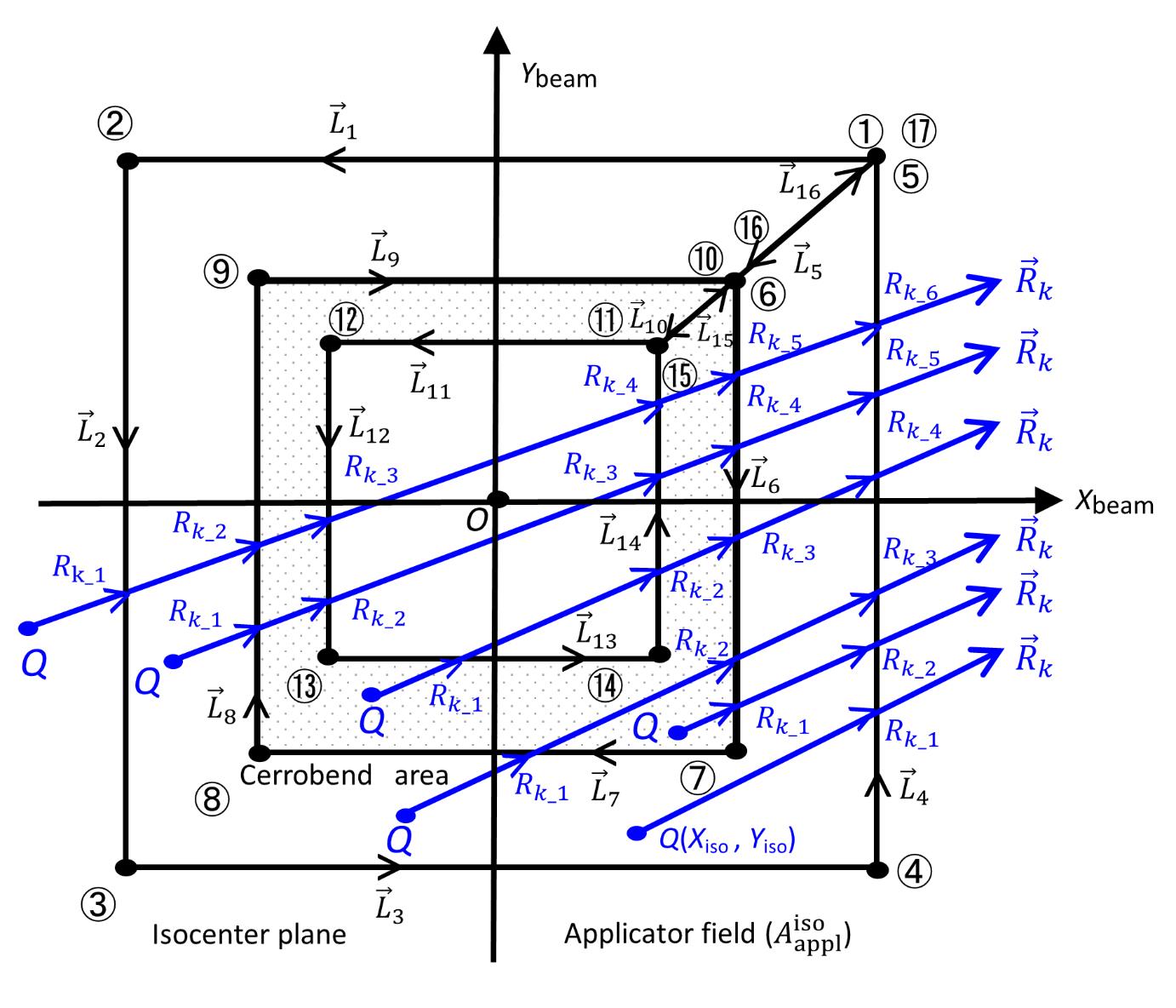
For one of the  lines (k=1,2,3,…) extending radically on the isocenter plane from point Q (refer to Figures 2-6, given later), if the corresponding line intersects the field border of the electron applicator or the cerrobend insert at distances of Rk_1, Rk_2, Rk_3, etc., measured from point Q, it is necessary to set the special factors of interest for Rk_i (i=1,2,3,…) as
 (Eq. 6)
Moreover, it has been found (Figures C1 (a) and (b)) that α(E)=1 is a good and simple model for any contaminant X-ray beam energy (E) and for any electron applicator field (). It should be noted that the present paper does not directly use the h0(E) function.
(i) When using Clarkson’s sector method, we assume that, on the isocenter plane, a square field with a side of S is equivalent to a circular field with a radius of  . The present paper utilizes this assumption for both the PDD function and the SF function taking the field size measured on the isocenter plane.
(j) For each energy E, the W-K MC dose datasets are expressed using the normalized valuation obtained when a common virtual accelerator is set up to deliver 1.0 Gy per 100 MU at a depth of dmax on the isocenter axis in water, where dmax is the depth at which the maximum dose caused by the electron-beam irradiation with an open electron applicator of =20×20 cm2 is yielded (this means that the W-K MC dose datasets are all expressed in Gy/100 MU for each electron beam). Conversely, the present analytical dose calculation is performed for contaminant X-ray beams, based on published radiotherapy X-ray PDD datasets. Therefore, when comparing the analytical and MC datasets for each combination of and E, we need to take into account the X-ray spectrum difference between the contaminant X-ray beam and the published radiotherapy PDD X-ray beam, and we should introduce a conversion factor of CFMC/PDD(Gy/100 MU/%) for setting both datasets at the same dose valuation level. However, the present study does not directly use the CFMC/PDD factor for the dose calculation.
(k) Under the assumption that the contaminant X-rays are all emitted from the point at a distance of SSDX=100 cm from the isocenter (O) along the isocenter axis (Figure 1), we may suppose that there is no change in PPD with SSD between the contaminant X-ray PDD function of SSDX=100 cm and the published radiotherapy X-ray PDD function [8, 9] with SSD0=100 cm (the following PDD functions are described under SSD0=SSDX=100 cm). For a given dose evaluation depth Z0, taking as a beam field on the isocenter plane, we let the published radiotherapy X-ray PDD function be expressed as PDD0=PDD0 (Z0,, E), and let the contaminant X-ray PDD function be expressed as PDDX=PDDX (Z0,, E).
(l) It has been found that the contaminant X-ray PDDX can be approximated as follows:
For Z0<Zmax (E)
 (Eq. 7)
letting  be the equivalent square field side of , where
 (Eq. 8)
 (Eq. 9)
Next for Z0<Zmax (E)
 (Eq. 10)
Here, the pair of Qa(E) and V0(E) and the pair of Qb(E) and β(E) are introduced to consider the X-ray spectrum change between the PDDX and PDD0 X-ray beams of energy E.
(m) Figure 2 shows two arrangements for point Q(Xiso, Yiso) on the isocenter plane. One is set in the field, and the other is outside the field. For the dose calculation relating to each Q point using Clarkson’s sector method, we take the line with an inclination angle θk radiating from point Q on the isocenter plane, setting θk=(k-1) Δθ0+ Δθ0/2 (k = 1 −360) with Δθ0 =2π/360 (radian), taken as anticlockwise rotation angles measured from the Xbeam axis direction.
(n) Based on the above preconditions, we describe how to calculate the dose for point P(Xcal, Ycal, Zcal ) by summing up each dose element (ΔD) obtained from the corresponding sector of  and Δθ0. Figure 2 shows the case containing no cerrobend insert (=0). Let
  (j=1-4) be the line vectors for the sides of the field, taking the rectangular field corners anticlockwise as ①,②,…,⑤.
First, we set point Q(Xiso, Yiso) inside the field, letting the line intersect with the field side of  as an example, and letting the distance between the point Q and the intersection point be Rk_1. Then, we can calculate the dose of ΔD as
ΔD(Xcal, Ycal, Zcal)
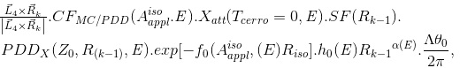 (Eq. 11)
where  and (Tcerrow=0, E)=1 (refer to (f)); SF(Rk_1) is the scatter factor (SF), evaluated using Rk_1 as the field radius (the SF can be set not as a function of E for MV photon beams [8]); and PDDX (Z0, Rk_1, E) is expressed using the field radius of Rk_1. It should be emphasized that the term h0(E)Rk_1αE is introduced to take into account the vague beam-field margin formed by the dual-foil system. We can then rewrite equation 11 as
ΔD(Xcal, Ycal, Zcal)=
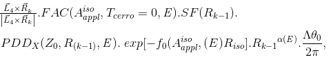 (Eq. 12)
with
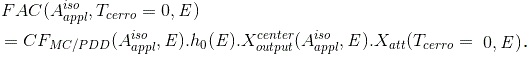 (Eq. 13)
As described later, we will attempt to evaluate the FAC function in one lump for a given irradiation condition.
(O) Second, we set point Q(Xiso, Yiso) outside the field (Figure 2). Then, the line concerns the sector dose calculation at two distances Rk_1 and Rk_2 from point Q. Let the line intersect with the electron applicator field sides as an example. We can then calculate the dose of ∆D as
ΔD(Xcal, Ycal, Zcal)=
 (Eq. 14)
where  and
and  . It should be emphasized that, when the line does not intersect with the field sides, we need to calculate the relational sector dose as ∆D(Xcal, Ycal, Zcal )=0. This fact shows one of the defects for the present sector method. However, it has been found that the α(E) function can effectively deal with such dose calculation defects, as shown in the off-axis dose (OAD) curves calculated in the next section.
 field, and the other is outside the field. The dose calculation relating to each Q(Xiso, Yiso) point is performed on the isocenter plane under Clarkson’s sector method using the line vectors of with Δθ0 and using the line vectors of (j=1-4) for the A_appl^iso field. The numbers ①,②,…,⑤ proceed anticlockwise from a corner of the field (the positions of ① and ⑤ are the same)..
(p) Figure 3 shows another irradiation case, in which a cerrobend insert with a hollow region in itself is set within an field. Then, we take points at distances of Rk_1, Rk_2, etc., measured from point Q(Xiso, Yiso) along the line, depending on the position. Figure 4 shows a case in which point Q is placed in the hollow region of the cerrobend insert, where (j=1, 2, …, 10) are straight continuous lines forming the cerrobend insert shape anticlockwise (the numbers ①,②,…,⑪ start from a point on the outside border of the cerrobend insert). Then, the dose ∆D from one sector of and Δθ0 within the cerrobend area can be similarly calculated as
ΔD(Xcal, Ycal, Zcal)=
 (Eq. 15)
with
 (Eq. 16)
Subsequently, we attempt to calculate the dose from the regions outside the cerrobend area.
 line starting from point Q(Xiso, Yiso), depending on the position for an irradiation case in which a cerrobend insert with a hollow region in itself is set within an field, and the other is outside the field..
 (j=1, 2, …, 10) are line vectors forming the cerrobend area, taken anticlockwise with the numbers ①,②,…,⑪ starting from a corner of the outside border of the cerrobend area (the positions of ① and ⑪ are at the same)..
Figure 5 shows how to take points at distances of Rk_1, Rk_2, etc., measured from point Q(Xiso, Yiso) along the line, depending on the position. Referring to Figure 6, in which point Q is set in the hollow region of the cerrobend insert, the dose ∆D from one sector of and Δθ0 can be calculated as
ΔD(Xcal, Ycal, Zcal)=
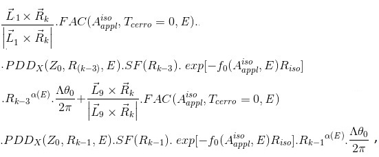 (Eq. 17)
where 
(q) Finally, we reassess the factor Xatt using equations 13 and 16. This is given by
 (Eq. 18)
 line starting from point Q(Xiso, Yiso) depending on the position. (j=1, 2, …, 16) are line vectors forming the area not covered with the cerrobend area, taken anticlockwise with the numbers ①,②,…,⑰ starting from a corner of the field (the positions of ① and ⑰ are at the same)..
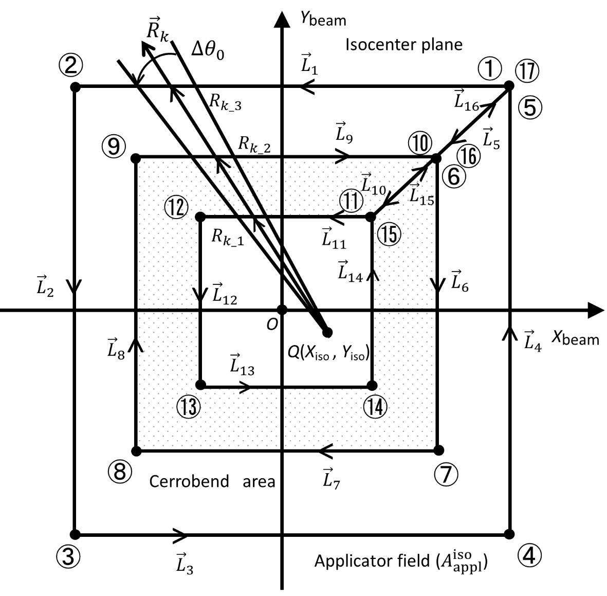 (j=1, 2, …, 16) and the numbers ①,②,…,⑰ are the same as in Figure 5..
Correspondence with the W-K MC dose datasets
The W-K MC dose datasets are produced using a common virtual accelerator for two MC simulation techniques: one is performed with BEAMnrc [10, 11] as the dose calculation simulation using a Cartesian voxel grid with the DOSXYZnrc code [12-14] as the phantom simulation (let the combination of these simulations be called the standard simulation technique); the other is performed using the MC-based dose calculation simulation in a commercial TPS.
The W-K MC dose datasets are performed in water phantoms for E=6, 12, and 18 MeV using =10×10 cm2,=10×10/14×14 cm2 (where 10×10 is the field produced using a cerrobend insert placed just inside the 14×14 applicator), and =20×20 cm2. The dose datasets are separated into depth dose (DD) curves and off-axis dose (OAD or profile-dose) curves, which are normalized with the dose obtained when the virtual accelerator is set up to deliver 1.0 Gy per 100 MU at the maximum dose depth (dmax) in water using =20×20 cm2 for each electron-beam energy (E). The dose datasets acquired using the standard simulation technique are composed of stepped curves of DD and OAD; and the dose datasets acquired using the commercial TPS are composed of dotted curves of DD and OAD. It should be noted that both the stepped and dotted datasets of OAD are classified as OAD profiles in the X and Y directions; however, the present paper does not refer to the OAD differences in the X and Y directions.
Results and discussionTop
The functions and constants used for each of the DD and OAD calculations were determined by trial and error. Table 1 summarizes values for the functions and constants, excluding α(E)=1, U0 ( ) as given by equation 8, and V0(E) as given by equation 9. Table 1 is classified into four groups: (a) the stepped curves of DD (Case-1 to -8), (b) the stepped curves of OAD (Case-9 to -16), (c) the dotted curves of DD (Case-17 to -24), and (d) the dotted curves of OAD (Case-25 to -32). For each case number, the corresponding reference datasets are given using figure numbers of the W-K MC dose work as follows:
Regarding the group (a),
Case-1 (=10×10 cm2, E=6 MeV) is for DD in Figure 3(a) under OAD in Figure 2(b);
Case-2 (=10×10 cm2, E=6 MeV) is for DD in Figure 3(a) under OAD in Figure 3(b);
Case-3 (=10×10 cm2, E=6 MeV) is for DD in Figure 3(a) under OAD in Figure 3(c);
Case-4 (=10×10/14×14 cm2, E=12 MeV) is for DD in Figure 5(a) under OAD in Figure 5(b);
Case-5 (=10×10/14×14 cm2, E=12 MeV) is for DD in Figure 5(a) under OAD in Figure 5(c);
Case-6 (=10×10 cm2, E=18 MeV) is for DD in Figure 3(d) under OAD in Figure 2(b));
Case-7 (=10×10 cm2, E=18 MeV) is for DD in Figure 3(d) under OAD in Figure 3(e);
Case-8 (=10×10 cm2, E=18 MeV) is for DD in Figure 3(d) under OAD in Figure 3(f).
Regarding the group (b),
Case-9 (=20×20 cm2, E=6 MeV) is for OAD (Zcal=5 cm) in Figure 2(b) under DD in Figure 3(a);
Case-10 (=10×10 cm2, E=6 MeV) is for OAD (Zcal=1 cm) in Figure 3(b) under DD in Figure 3(a);
Case-11 (=10×10 cm2, E=6 MeV) is for OAD (Zcal=5 cm) in Figure 3(c) under DD in Figure 3(a);
Case-12 (=10×10/14×14 cm2, E=12 MeV) is for OAD (Zcal=2 cm) in Figure 5(b) under DD in Figure 5(a);
Case-13 (=10×10/14×14 cm2, E=12 MeV) is for OAD (Zcal=10 cm) in Figure 5(c) under DD in Figure 5(a);
Case-14 (=20×20 cm2, E=18 MeV) is for OAD (Zcal=15 cm) in Figure 2(b) under DD in Figure 3(d);
Case-15 (=10×10 cm2, E=18 MeV) is for OAD (Zcal=3 cm) in Figure 3(e) under DD in Figure 3(d));
Case-16 (=10×10 cm2, E=18 MeV) is for OAD (Zcal=15 cm) in Figure 3(f) under DD in Figure 3(d).
Regarding the group (c),
Case-17 (=10×10 cm2, E=6 MeV) is for DD in Figure 3(a) under OAD in Figure 2(b);
Case-18 (=10×10 cm2, E=6 MeV) is for DD in Figure 3(a) under OAD in Figure 3(b);
Case-19 (=10×10 cm2, E=6 MeV) is for DD in Figure 3(a) under OAD in Figure 3(c);
Case-20 (=10×10/14×14 cm2, E=12 MeV) is for DD in Figure 5(a) under OAD in Figure 5(b);
Case-21 (=10×10/14×14 cm2, E=12 MeV) is for DD in Figure 5(a) under OAD in Figure 5(c);
Case-22 (=10×10 cm2, E=18 MeV) is for DD in Figure 3(d) under OAD in Figure 2(b);
Case-23 (=10×10 cm2, E=18 MeV) is for DD in Figure 3(d) under OAD in Figure 3(e);
Case-24 (=10×10 cm2, E=18 MeV) is for DD in Figure 3(d) under OAD in Figure 3(f).
Regarding the group (d),
Case-25 (=20×20 cm2, E=6 MeV) is for OAD (Zcal=5 cm) in Figure 2(b) under DD in Figure 3(a);
Case-26 (=10×10 cm2, E=6 MeV) is for OAD (Zcal=1 cm) in Figure 3(b) under DD in Figure 3(a);
Case-27 (=10×10 cm2, E=6 MeV) is for OAD (Zcal=5 cm) in Figure 3(c) under DD in Figure 3(a);
Case-28 (=10×10/14×14 cm2, E=12 MeV) is for OAD (Zcal=2 cm) in Figure 5(b) under DD in Figure 5(a);
Case-29 (=10×10/14×14 cm2, E=12 MeV) is for OAD (Zcal=10 cm) in Figure 5(c) under DD in Figure 5(a);
Case-30 (=20×20 cm2, E=18 MeV) is for OAD (Zcal=15 cm) in Figure 2(b) under DD in Figure 3(d);
Case-31 (=10×10 cm2, E=18 MeV) is for OAD (Zcal=3 cm) in Figure 3(e) under DD in Figure 3(d);
Case-32 (=10×10 cm2, E=18 MeV) is for OAD (Zcal=15 cm) in Figure 3(f) under DD in Figure 3(d).
Table 1 also lists values of Zmax(E), Applicator ( & =equivalent square field side of ), Qa(E), Qb(E), β(E), f0E), FAC(, =0, E), FAC(, >0,E), and (≥0,E).
By analyzing the datasets of the stepped curves of DD and OAD (Case-1 to -16) regarding the functions of Qa(E), Qb(E), β(E), f0E, we constructed the following regression equations:
 (Eq. 19)
 (Eq. 20)
 (Eq. 21)
 (Eq. 22)
Conversely, for the FAC function, we used and E as variables (letting be defined as the equivalent square field side of ). By analyzing the FAC datasets of Case-1 to -16, we constructed a FAC regression function of
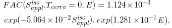 (Eq. 23)
Similarly, for the dotted curves of DD and OAD under Case-17 to -32, we built the following regression equations:
 (Eq. 24)
 (Eq. 25)
 (Eq. 26)
 (Eq. 27)
 (Eq. 28)
These regression functions may be useful for estimating reasonable values for the corresponding functions for given irradiation conditions. Details are described in Appendix A. Further in Appendix B, we refer to detailed results for calculated and MC-based DD and OAD datasets; and in Appendix C, we refer to the working of the function (E).
| Case-no. E(MeV) |
Zmax (E) cm | Applicator / cm2 |
Qa(E) | Qb(E) | β(E) | f0(E) (cm-1) | FAC(, )(for =0) |
FAC (, )(for >0) |
(, )(for ≥0) |
| Case-1 E=6 MeV |
1.5 | 10 × 10 =10.5 cm) |
1.000 | 9.428E-04 | 1.946 | 2.638E-03 | 1.287E-05 | no existing | 1 |
| Case-2 E=6 MeV |
1.5 | (10×10 =10.5 cm) |
1.000 | 9.428E-04 | 1.946 | 4.411E-03 | 1.287E-05 | no existing | 1 |
| Case-3 E=6 MeV |
1.5 | (10×10 =10.5 cm) |
1.000 | 9.428E-04 | 1.946 | 3.819E-02 | 1.287E-05 | no existing | 1 |
| Case-4 E=12 MeV |
2.6 | (10×10 =14.7 cm) |
1.043 | 1.097E-02 | 1.097 | 4.401E-02 | 3.123E-05 | 1.875E-05 | 0.600 |
| Case-5 E=12 MeV |
2.6 | (10×10 =14.7 cm) |
1.043 | 1.097E-02 | 1.097 | 3.264E-02 | 3.205E-05 | 1.722E-05 | 0.537 |
| Case-6 E=18 MeV |
3.2 | (10×10 =10.5 cm) |
1.100 | 3.000E-03 | 1.501 | 4.898E-02 | 5.993E-05 | no existing | 1 |
| Case-7 E=18 MeV |
3.2 | (10×10 =10.5 cm) |
1.100 | 3.000E-03 | 1.501 | 3.853E-02 | 5.993E-05 | no existing | 1 |
| Case-8 E=18 MeV |
3.2 | (10×10 =10.5 cm) |
1.100 | 3.000E-03 | 1.501 | 5.305E-02 | 5.993E-05 | no existing | 1 |
| Case-no. E(MeV) |
Zmax (E) cm | Applicator / cm2 |
Qa(E) | Qb(E) | β(E) | f0(E) (cm-1) | FAC(, )(for =0) |
FAC (, )(for >0) |
(, )(for ≥0) |
| Case-9 E=6 MeV |
1.5 | 20×20 =21.1 cm) |
1.000 | 9.428E-04 | 1.946 | 2.638E-03 | 6.495E-06 | no existing | 1 |
| Case-10 E=6 MeV |
1.5 | (10×10 =10.5 cm) |
1.000 | 9.428E-04 | 1.946 | 4.411E-03 | 1.335E-05 | no existing | 1 |
| Case-11 E=6 MeV |
1.5 | (10×10 =10.5 cm) |
1.000 | 9.428E-04 | 1.946 | 3.819E-02 | 1.433E-05 | no existing | 1 |
| Case-12 E=12 MeV |
2.6 | (10×10/ 14×14 =14.7 cm) |
1.043 | 1.097E-02 | 1.097 | 2.739E-02 | 3.084E-05 | 1.852E-05 | 0.600 |
| Case-13 E=12 MeV |
2.6 | (10×10/ 14×14 =14.7 cm) |
1.043 | 1.097E-02 | 1.097 | 4.287E-02 | 3.126E-05 | 1.679E-05 | 0.537 |
| Case-14 E=18 MeV |
3.2 | (20×20 =21.1 cm) |
1.100 | 3.000E-03 | 1.501 | 4.898E-02 | 3.282E-05 | no existing | 1 |
| Case-15 E=18 MeV |
3.2 | (10×10 =10.5 cm) |
1.100 | 3.000E-03 | 1.501 | 3.853E-02 | 6.424E-05 | no existing | 1 |
| Case-16 E=18 MeV |
3.2 | (10×10 =10.5 cm) |
1.100 | 3.000E-03 | 1.501 | 5.305E-02 | 6.427E-05 | no existing | 1 |
| Case-no. E(MeV) |
Zmax (E) cm | Applicator / cm2 |
Qa(E) | Qb(E) | β(E) | f0(E) (cm-1) | FAC(, )(for =0) |
FAC (, )(for >0) |
(, )(for ≥0) |
| Case-17 E=6 MeV |
1.5 | 10×10 =10.5 cm) |
1.400 | 3.428E-04 | 2.396 | 2.763E-02 | 1.291E-05 | no existing | 1 |
| Case-18 E=6 MeV |
1.5 | (10×10 =10.5 cm) |
1.400 | 3.428E-04 | 2.396 | 3.017E-02 | 1.291E-05 | no existing | 1 |
| Case-19 E=6 MeV |
1.5 | (10×10 =10.5 cm) |
1.400 | 3.428E-04 | 2.396 | 2.107E-02 | 1.291E-05 | no existing | 1 |
| Case-20 E=12 MeV |
2.6 | (10×10/ 14×14 =14.7 cm) |
1.200 | 1.780E-02 | 1.110 | 2.975E-02 | 3.042E-05 | 1.319E-05 | 0.434 |
| Case-21 E=12 MeV |
2.6 | (10×10/ 14×14 =14.7 cm) |
1.200 | 1.780E-02 | 1.110 | 2.477E-02 | 3.182E-05 | 1.010E-05 | 0.318 |
| Case-22 E=18 MeV |
3.2 | (10×10 =10.5 cm) |
0.957 | 7.903E-02 | 0.677 | 5.659E-02 | 7.730E-05 | no existing | 1 |
| Case-23 E=18 MeV |
3.2 | (10×10 =10.5 cm) |
0.957 | 7.903E-02 | 0.677 | 1.963E-02 | 7.730E-05 | no existing | 1 |
| Case-24 E=18 MeV |
3.2 | (10×10 =10.5 cm) |
0.957 | 7.903E-02 | 0.677 | 3.751E-02 | 7.730E-05 | no existing | 1 |
| Case-no. E(MeV) |
Zmax (E) cm | Applicator / cm2 |
Qa(E) | Qb(E) | β(E) | f0(E) (cm-1) | FAC(, )(for =0) |
FAC (, )(for >0) |
(, )(for ≥0) |
| Case-25 E=6 MeV |
1.5 | 20×20 =21.1 cm) |
1.400 | 3.428E-04 | 2.396 | 2.763E-02 | 7.429E-06 | no existing | 1 |
| Case-26 E=6 MeV |
1.5 | (10×10 =10.5 cm) |
1.400 | 3.428E-04 | 3.017E-02 | 4.411E-03 | 1.463E-05 | no existing | 1 |
| Case-27 E=6 MeV |
1.5 | (10×10 =10.5 cm) |
1.400 | 3.428E-04 | 2.396 | 2.107E-02 | 1.347E-05 | no existing | 1 |
| Case-28 E=12 MeV |
2.6 | (10×10/ 14×14 =14.7 cm) |
1.200 | 1.780E-02 | 1.110 | 2.868E-02 | 2.963E-05 | 1.285E-05 | 0.434 |
| Case-29 E=12 MeV |
2.6 | (10×10/ 14×14 =14.7 cm) |
1.200 | 1.780E-02 | 1.110 | 2.752E-02 | 3.199E-05 | 1.016E-05 | 0.318 |
| Case-30 E=18 MeV |
3.2 | (20×20 =21.1 cm) |
0.957 | 7.903E-02 | 0.677 | 5.659E-02 | 4.469E-05 | no existing | 1 |
| Case-31 E=18 MeV |
3.2 | (10×10 =10.5 cm) |
0.957 | 7.903E-02 | 0.677 | 1.963E-02 | 7.577E-05 | no existing | 1 |
| Case-32 E=18 MeV |
3.2 | (10×10 =10.5 cm) |
0.957 | 7.903E-02 | 0.677 | 3.751E-02 | 8.867E-05 | no existing | 1 |
ConclusionTop
We attempted to develop an analytical method for 3-dimensional (3D) calculation of the contaminant X-ray dose in water caused by clinical electron-beam irradiation in light of the two groups of Monte Carlo (MC) datasets reported by Wieslander and Knöös (2006). The analytical method is based on Clarkson’s sector method. However, the original sector method was modified to take into account the following terms: (a) the vague beam-field margins formed by the dual-foil system; (b) the in-air dose distribution of the contaminant X-ray beam; (c) the difference between the X-ray spectrum used for constructing the contaminant X-ray PDD datasets and that used for constructing the published radiotherapy X-ray PDD datasets; and (d) the contaminant X-ray attenuation for the cerrobent insert, if any. We can conclude that the analytical method can achieve accurate dose calculations, even for beams with cerrobent inserts. In particular, it should be emphasized that the analytical method can give almost the same calculation results as the MC-based dose calculation algorithm in a commercial TPS.
Acknowledgements
We would like to thank Editage (www.editage.com) for English language editing.
Conflicts of interest
This study was carried out in collaboration with Technology of Radiotherapy Corporation, Tokyo, Japan. This sponsor had no control over the interpretation, writing, or publication of this work.
Supplementary dataTop
ReferencesTop
[1]Khan FM. The physics of radiation therapy; 3rd edition. Philadelphia, USA; 2003.Website
[2]Mahdavi M, Mahdavi SRM, Alijanzadeh H, Zabihzadeh M. Comparing the measurement value of photon contamination absorbed dose in electron beam field for varian clinical accelerator. The IUP Journal of Physics. 2011; 4(3): 7−11.Article
[3]Geyer P, Baus WW, Baumann M. Portal verification of high energy electron beams using their photon contamination by film-cassette systems. Strahlenther Onkol. 2006; 182(1): 37−44.Article Pubmed
[4]Sorcini BB, Hyödynmaa S, Brahme A. Quantification of mean energy and photon contamination for accurate dosimetry of high-energy electron beams. Phys Med Biol. 1997; 42(10):1849−1873.Article Pubmed
[5]Zhu TC, Das IJ, Bjärngard BE. Characteristics of bremsstrahlung in electron beams. Med Phys. 2001; 28(7): 1352−1358.Article
[6]Wieslander E, Knöös T. A virtual linear accelerator for verification of treatment planning systems. Phys. Med. Biol. 2000; 45(10): 2887–2896.Article Pubmed
[7]Wieslander E, Knöös T. A virtual-accelerator-based verification of a Monte Carlo dose calculation algorithm for electron beam treatment planning in homogeneous phantoms. Phys Med Biol. 2006; 51(6):1533–1544.Article Pubmed
[8]Aird EGA, Burns JE, Day MJ, Duane S, Jordan TJ, et al. BJR Supplement 25: Central axis depth dose data for use in radiotherapy (1996). British Institute of Radiology, 36 Portland Place, London W1N 4AT. London, 1996.
[9]Japan Society of Medical Physics. Standard dosimetry of absorbed dose in external beam radiotherapy (1972).
[10]Rogers DWO, Faddegon BA, Ding GX, Ma C-M, Wei J, et al. BEAM: a Monte Carlo code to simulate radiotherapy treatment units. Med Phys. 1995; 22(5):503–524.Article Pubmed
[11]Rogers DWO, Ma C-M, Walters B, Ding GX, Sheikh-Bagheri D, et al. BEAM Users Manual: NRC Report PIRS-0509A (rev G), 2002.
[12]Kawrakow I. Accurate condensed history Monte Carlo simulation of electron transport: I. EGSnrc, the new EGS4 version. Med Phys. 2000; 27(3):485–498.Article Pubmed
[13]Kawrakow I, Rogers DWO. The EGSnrc system, a status report. Advanced Monte Carlo for radiation physics, particle transport simulation and applications: Proc. Monte Carlo 2000 Meeting ed. A Kling, F Barao, M Nakagawa, L T´avora, P Vaz (Berlin: Springer), 2001.Article
[14]Walters BRB, Rogers DWO. DOSXYZnrc Users Manual: NRC Report PIRS-794, 2002.
 Copyright
© 2012-2025 NobleResearch Group. All Rights Reserved
Copyright
© 2012-2025 NobleResearch Group. All Rights Reserved