Original researchOpen Access

AbstractTop

Purposes: This paper highlights a 10-MV X-ray convolution dose calculation method in water using primary and scatter dose kernels formed for energy bins of X-ray spectra reconstructed as a function of the off-axis distance for a linear accelerator equipped with pairs of upper and lower jaws, a multileaf collimator (MLC) and a wedge filter. Methods: The reconstructed X-ray spectra set was composed of 11 energy bins. To estimate the in-air beam intensities at points on the isocenter plane for an MLC field, we employed an MLC leaf-field output subtraction method, using an extended radiation source on each of the X-ray target and the flattening filter as well as simplified two-dimensional plates to simulate the three-dimensional jaws and MLC structures. A special correction factor was introduced for nonuniform incident beam intensities, particularly produced at MLC fields. The in-phantom dose calculation was performed by treating the phantom, the wedge filter, the wedge holder and the MLC as parts of a unified irradiated body, where we proposed to use a special factor for the density scaling theorem within the unified irradiated body. Conclusions: The phantom dose was generally separated into nine dose-components: The primary and scatter dose-components produced in the phantom; the primary and scatter dose-components emanating from the wedge, the wedge holder and the MLC; and the electron contamination dose-component. From the calculated and measured percentage depth dose (PDD) and off-center ratio (OCR) datasets, we may conclude that the convolution method can achieve accurate dose calculations even under MLC and/or wedge filtration.

Keywords: convolution method; X-ray spectra; dose kernels; wedge; multileaf collimation; MLC leaf-field output subtraction

Research highlightsTop

Convolution methods are convenient for three-dimensional (3D) dose calculations, especially for an irregular-beam field with a non-uniform incident-beam intensity distribution. For a convolution method, we performed theoretical and experimental studies on 10-MV X-ray dose calculations in water phantoms with multileaf collimation (MLC) and/or wedge filtration using a linear accelerator equipped with a pair of upper jaws, a pair of lower jaws, an MLC and a wedge filter. The in-phantom dose calculation was performed by treating the phantom, the wedge filter, the wedge holder and the MLC as parts of a unified irradiated body. We can conclude that the convolution method can achieve accurate dose calculations even under MLC and/or wedge filtration.

IntroductionTop

Megavoltage X-ray beams from linear accelerators are used for radiation therapy. The X-ray radiation produced in the X-ray target pass through a flattening filter that is symmetric with respect to the isocenter axis. The flattening filter makes the beam intensity distribution relatively uniform across the field. The filter is thickest in the middle and tapers off toward the edges; therefore, the X-ray spectrum is a function of the off-axis distance (radiation softening becomes more pronounced with increasing off-axis distance).

The dose at a point in a medium irradiated by an X-ray beam can be separated into three components. One is the primary dose, arising directly from primary photons that have not interacted with the medium before reaching the point. Another is the dose from scattered radiation originating from all points hit by primary photons in the medium. The last is the contamination dose, caused by electrons from the treatment head and air volume. With model-based algorithms, one can calculate the primary, scatter and contamination dose components separately. Convolution (or superposition) methods are in the class of model-based algorithms. They are convenient for three-dimensional (3D) dose calculations, especially for an irregular-beam field with a nonuniform incident-beam intensity distribution. As reviewed by Ahnesjö and Aspradakis [1], there are two kinds of convolution methods: one is a method that uses pencil-beam kernels, and the other is a method that uses point-dose kernels.

With respect to the latter convolution method, its numerical convolution is also called “the collapsed cone convolution” [2]. The present paper deals with a kind of collapsed cone convolution; however, it is to be emphasized that the dose calculation is performed using multiple primary- and scatter-dose kernels that are formed with the use of X-ray spectra reconstructed [3, 4] as a function of the off-axis distance.

For accurate primary and scatter dose calculations using convolution methods, Iwasaki [5] stipulated that the following four irradiation conditions be met: (a) a nondivergent beam, (b) a homogeneous phantom, (c) a beam attenuation coefficient along ray lines that is not a function of the depth and off-axis distance, and (d) an incident beam intensity that is uniform within the irradiation field and zero outside it. We have not yet dealt with the condition described in (a). Iwasaki, et al. [6] and Kimura, et al. [7] dealt with the condition described in (b) using inhomogeneous phantoms, proposing a correction factor for calculation of the primary dose within thorax-like phantoms, and also dealt with the condition described in (c) using X-ray spectra reconstructed as a function of the off-axis distance. In the present paper, we proposed a special correction factor for nonuniformity of the incident beam intensity described in the above (d) using multileaf collimator (MLC) and/or wedge fields. Because the MLC and wedge devices are usually made of high-Z materials, they can induce large changes in the incident beam intensity (also including the X-ray spectrum changes). The dose calculation simulations are performed using 10-MV X-ray beams, focusing on percentage depth dose (PDD) and off-center ratio (OCR) datasets in water phantoms.

Materials and methodsTop

The physical parameters of the materials used in this study were evaluated using data tables published by Hubbell [8]. We used 10-MV X-ray beams from a linear accelerator (CL-2100C; Varian Medical Systems, Palo Alto, CA, USA). The treatment head contains pairs of upper and lower jaws: upper-1, -2 and lower-1, -2 (tungsten alloy) as the jaw collimator which is able to form a jaw field ≤ 40 × 40 cm² on the isocenter plane 100 cm distant from the source (S) (or the X-ray target). The treatment head also features an MLC (Millennium 120 Leaf; Varian Medical Systems) under the jaw-collimator device. Each leaf moves in the same direction as the lower jaws. We used wedge filters supplied by the manufacturer that are designed to be installed directly on the treatment head. The wedge filters, made of steel or lead alloys, form isodose angles of 15°, 30°, 45° and 60° in water and are mounted on an acrylic plate (wedge holder). Figure 1 diagrams the treatment head with an installed wedge. We let A_jaw and A_MLC denote the jaw and MLC fields, respectively, measured on the isocenter plane.

Figure 1 The treatment head is composed of a source (S), a pair of upper jaws, a pair of lower jaws, and pairs of MLC leaves. A wedge filter can be placed on the treatment head. The orthogonal coordinate system with axes of X_beam, Y_beam and Z_beam setting the origins at the isocenter (O) was used for the dose calculation model.

Symbols and units We use the following symbols and units in this paper: the spectra-related energies (E_N and ΔE_N) are expressed in MeV; the normalized set of reconstructed energy fluences (Ψ's) is expressed in MeV^-1; the total in-air beam energy fluence is expressed in J/cm²; the linear attenuation coefficients (e.g., μ_water, μ_phan, μ_wedge, μ_MLC, ) for media are expressed in cm^-1); the lengths (Ξ, Η, ξ, η, R, r, R₀, etc.) are expressed in cm; the position vectors () are expressed in cm; the primary and scatter dose components are expressed in Gy; the beam water collision kerma (or the primary water collision kerma) components are expressed in Gy; the dose kernels (H_1,2, K_1,2, h_phan, h_wedge, h_MLC, k_phan, k_wedge, k_MLC, etc.) are expressed in cm^-3; the volume element (ΔV) is expressed in cm³; and the area element (ΔS) is expressed in cm².

Theoretical studies We tried to calculate the dose at a point generally in an inhomogeneous phantom by treating the phantom, the wedge filter, the wedge holder and the MLC as parts of a unified irradiated body. For this calculation model, we used an orthogonal coordinate system of (X_beam, Y_beam, Z_beam) (Figures 1 and 2), setting the origin (O) at the isocenter. We denote the Z_beam axis as the line connecting the source (S) and the origin (O), coinciding with the isocenter axis, and assume that the X_beam and Y_beam axes perpendicularly intersect the upper- and lower-jaw field edges, respectively, on the isocenter plane (Z_beam = 0 cm), calling this the “beam coordinate system”. The MLC leaves move parallel to the Y_beam axis, in the same direction as that of the lower jaws. To calculate the expressions of equations 1−3 described in the following text to evaluate the dose at a point P(X_c, Y_c, Z_c) in the phantom (Figure 2), we use two other coordinate systems in addition to the beam coordinate system (X_beam, Y_beam, Z_beam): one is the orthogonal coordinate system (x_v, y_v, z_v) with the origin at point P (it should be noted that the (x_v, y_v, z_v) coordinate system just coincides with the (X_beam, Y_beam, Z_beam) coordinate system when point P coincides with the isocenter (O); and the other is the polar coordinate system (r', Φ, θ) directly associated with the (x_v, y_v, z_v) coordinate system.

Figure 2 (a) Diagram showing how to calculate the dose at point P in the phantom, where wedge and MLC devices are generally used; the primary and scatter doses emanate from the volume elements (ΔV’s) in the phantom, wedge filter, wedge holder and MLC (unified irradiated body); the electron contamination dose emanates from the area element (ΔS) on the phantom surface; are the position vectors; and θ_phan, θ_wedge, θ_{w_hold}, θ_MLC and θ_s are the angles (it should be emphasized that the (x_v, y_v, z_v) coordinate system becomes the (X_beam, Y_beam, Z_beam) coordinate system when point P coincides with the isocenter (O); (b) Diagram showing how to determine the effective point within a volume element (ΔV) in the phantom as with f_V = 0.415 for primary dose calculations, and with f_V = 0.01 for scatter dose calculations, also showing how to set OPF_J data (J = 1,2,....,J_max(= 27))on the isocenter plane.

Dose calculation principle
The dose calculation was performed using a convolution method that utilizes special types of in-water primary and scatter dose kernels (H_1,2 and K_1,2 (see Appendix A)), formed for the energy bins of X-ray spectra [3, 4] reconstructed as a function of the off-axis distance. It should be noted that the usual number of energy bins is approximately ten, and that the reconstructed X-ray spectra can reasonably be applied [4] to media with a wide range of effective Z numbers (e.g., from water to lead). When applying the density scaling theorem [9-11] to the in-water primary and scatter dose kernels again under the conditions that the phantom, wedge filter, wedge holder and MLC are treated as parts of a unified irradiated body, the use of the relative electron density (ρe) is not feasible. This is because the effective Z numbers of the media within the unified irradiated body are quite different from one another, depending on the energy bins of the reconstructed X-ray spectra. Thus, we propose to use a factor of μ_med/ μ_water (the relative attenuation factor) for the medium of each volume element within the unified irradiated body, where μ_med and μ_water are the linear attenuation coefficients of the volume element material and water, respectively, and are determined by each of the energy bins of the reconstructed X-ray spectra. For the volume elements existing along a line connecting two points, we propose to use the mean relative attenuation factor, instead of using the mean relative electron density . It should be noted that the linear attenuation coefficients μ_med, μ_water and generally change with the energy bin of the reconstructed X-ray spectra, whereas ρe or does not. In addition, for water-like media, we can assume ρe = μ_med/ μ_water and for any energy bin. This method of using the linear attenuation coefficients may be effective for handling the scatter dose kernels. However, it may not be effective for handling the primary dose kernels because the primary dose is caused by the secondary electrons generated by the interaction between the volume element and the primary photons. The secondary electrons do not have a strong relationship with photon attenuation from the standpoint of energy deposition in media.

Figure 2 also shows a quadrangular pyramid in polar coordinates, whose apex is situated at point P. It shows how to calculate the primary, scatter and electron contamination doses delivered to point P, where the primary and scatter doses arise from the volume elements (ΔV’s) in the unified irradiated body; and the electron contamination dose arises from the area element ΔS. Regarding to the volume elements (ΔV's) and area elements (ΔS's), we employed a series of θ, Δθ, Φ, ΔΦ, r' data (see Appendix B). For the convolution dose calculation, (a) we used a set of X-ray spectra reconstructed as a function of the off-axis distance, letting the bin energies be E_N (N = 1, 2,....., N_max with N_max ≅ 10) for each off-axis distance; (b) we used primary dose kernels (h_phan, h_wedge, h_{w_hold} and h_MLC) and scatter dose kernels (k_phan, k_wedge, k_{w_hold} and k_MLC) as a function of E_N for the volume and area elements, where these dose kernels are rebuilt from the in-water primary and scatter dose kernels (H_1,2 and K_1,2); and (c) we estimated values of as a function of E_N for each of the volume and area elements.

For dose calculation generally under the presence of the MLC and a wedge filter, we divided the dose to point P into nine components: (a) the primary and scatter doses produced in the phantom; (b) the primary and scatter doses emanating from the wedge filter; (c) the primary and scatter doses emanating from the wedge holder; (d) the primary and scatter doses emanating from the MLC; and (e) the contamination dose D_cont caused by the electrons emanating from the treatment head and the air volume.

It should be noted that this calculation method does not strictly take into account the primary and scatter doses due to the secondary electrons and scattered photons, respectively, produced in the upper and lower jaws. Instead, it treats the radiation reflected from the jaws as a small increase in the in-air beam intensity using a jaw radiation reflection factor [6] that lies outside the jaw field, as described by a Monte Carlo simulation model [12] stating that the photons scattered from the jaws can be ignored when estimating the in-air beam intensity within the jaw field.

Within the unified irradiated body, we set the beam water collision kerma to act on the dose kernel at each ΔV or ΔS element point. When the beam water collision kerma should be determined based on the open jaw field without the MLC device, we denote it as . When the beam water collision kerma should be determined based on the open MLC field under a given jaw field, we denote it as .

Next, we describe the dose calculation approaches using position vectors, generally taking an irradiation case in which both wedge and MLC devices are installed in a jaw field (Figure 2a). We let L_c denote the position vector to a dose calculation point P, drawn from the source (S); and denote the position vectors to volume elements ΔV's in the phantom, wedge filter, wedge holder and MLC, respectively, drawn from the source (S); and L_Δs denote the position vector to an area element (ΔS) on the phantom surface, drawn from the source (S). Then the primary, scatter and electron contamination dose calculations are performed using the follow approaches.

(a) The primary dose calculation approach:

where express the beam water collision kermas at the corresponding volume elements (ΔV’s), respectively, in the phantom and in the wedge or MLC device (equations 40-42, 46).

(b) The scatter dose calculation approach:

(c) The contamination dose calculation approach:

where express the beam water collision kerma at the corresponding phantom surface element (ΔS) (equation 43); ΔS is defined as the size of the area element on the phantom surface, which faces the source (S) without interception by the phantom; θ_S is the angle between the normal vector line on the ΔS surface and the negative vector of ; G(A_jaw) expresses the electron contamination factor as a function of the jaw field (A_jaw) [6, 7]. Γ₁ and Γ₂ are introduced to improve the G function, which can apply only to open jaw fields and only to electrons streaming along the ray lines emanating from the source (S).

Γ₁ represents the degree of attenuation of the contaminant electrons when penetrating the MLC and wedge filter along the position vector L_ΔS. Let Γ₁ be formulated using penetration features of the secondary electrons produced by E_N photons as

where H₁(Ξ, R; E_N) expresses the in-water forward primary dose kernel to point (Ξ, R) produced by E_N photons (refer to Appendix A); and T_eff (E_N) is the total effective thickness for the MLC and wedge devices, evaluated along the position vector L_ΔS as a function of E_N. It is calculated as

where µ_MLC(E_N), µ_wedge(E_N), µ_{w_hold}(E_N) and µ_water(E_N) are the linear attenuation coefficients of the MLC, wedge filter, wedge holder and water, respectively, for E_N photons; and T_MLC, T_wedge and T_{w_hold} are the thicknesses of the MLC, wedge filter and wedge holder, respectively, measured along the position vector L_ΔS.

Γ₁ is introduced to improve the accuracy of the calculation at points very near the phantom surface [7], to take into account the dose delivered by the contaminant electrons coming across the ray lines. For phantoms constructed of water-like media, we express Γ₂ as

Where is the relative electron density averaged between point P and the ΔS center (however, it has been found [13, 15] that the contamination dose does not vary simply in proportion to the beam water collision kerma of .

In regard to the calculated dose to point P(X_C, Y_C, Z_C) in the phantom (Figure 2), it can be understood that the primary and scatter doses emanating from the volume elements in the phantom are generally composed of forward and backward dose components, that the primary and scatter doses emanating from volume elements in the wedge and MLC devices are composed only of forward dose components because these devices are placed relatively far above the phantom, and that the contamination dose is generally composed of forward and backward dose components. Appendix A defines in-water primary and scatter dose kernels as H₁(Ξ, R; E_N), H₂(Η, R; E_N), K₁(Ξ, R; E_N) and K₂(Ξ, R; E_N) using orthogonal coordinates (Ξ, R) and (H, R) for incident E_N photons.

Next, we examine the dose kernels of h_phan, h_wedge, h_{w_hold}, h_MLC, k_phan, k_wedge, k_{w_hold} and k_MLC (equations 1-3) used in the unified irradiated body. According to the aforementioned density scaling theorem, the coordinates of ξ, η, r, ξ_s, η_s and r_s shown in Figure 3 can be converted to the in-water coordinates as:

Then, the dose kernels in equations 1-3 can be evaluated by employing the in-water dose kernels (H_1,2 and K_1,2 ) as follows (also refer to the angles of θ_phan, θ_S, θ_wedge, θ_{w_hold} and θ_MLC in Figure 2):
(a) h_phan in equation 1 is one of the following two kernels:

where is evaluated along the line connecting P and the effective point within the ΔV element; and F_hetero is a correction factor [6, 7] for phantom heterogeneity. This correction factor is simply used only for forward primary dose calculations, not as a function of E_N. We should set F_hetero = 1 for homogeneous phantoms.

(b) k_phan in equation 2 is one of the following two kernels:

(c) h_phan in equation 3 is one of the following two kernels:

where is evaluated along the line connecting P and the center of ΔS.

(d) h_wedge and k_wedge (used as θ_wedge < π/2) in equations 1 and 2 are, respectively,

where F_{wedge_p} and F_{wedge_s} are the correction factors, respectively, for the calculation of the primary and scatter dose components, not as a function of E_N. We express them as

with , where α_{wedge_p} = 2.5 × 10^-2, β_{wedge_p} = 0.5, α_{wedge_p} = 7.0 × 10^-8, β_{wedge_p} = 0.5 and γ_{wedge_s} = 50 for each of the 15°, 30°, 45° and 60° wedges (wedge types 1–4) (these values, without units, were derived by comparing the calculated and measured dose datasets).

(e) h_{w_hold} and k_{w_hold} (used as θ_{w_hold} < π/2) in equations 1 and 2 are, respectively,

(f) h_MLC and k_MLC (used as θ_MLC < π/2) in equations 1 and 2 are, respectively,

where F_{MLC_p} and F_{MLC_s} are the correction factors, respectively, for the calculation of the primary and scatter dose components emanating from the MLC, not as functions of E_N. We express them as

with , where we let α_{MLC_p} = 1 × 10^-3, β_{MLC_p} = 1.5, α_{MLC_s} = 100, β_{MLC_s} = 1.5 and γ_{MLC_s} = 1.0 (these values without units were derived by comparing the calculated and measured dose datasets).

Figure 3 (a) Diagram showing how to calculate the primary and scatter doses at point P(X_C, Y_C, Z_C) in a phantom. Point O_p is situated at the middle of the line connecting the source (S) and point P. A sphere is drawn with the diameter of SP, with the center set at point O_p. Points (ξ, r) and (η, r) are, respectively, inside and outside the sphere; (b) Diagram showing how to calculate the contamination dose at point P(X_C, Y_C, Z_C) in a phantom. Point O_p is situated at the middle of the line connecting the source (S) and point P. A sphere is drawn with the diameter of SP, with the center set at point O_p. Points (ξ_s, r_s) and (η_s, r_s) are, respectively, inside and outside the sphere.

Modeling the jaw collimator, MLC and wedge devices
The jaw collimator, MLC and wedge devices are 3D objects (Figure 4a). However, to simplify the calculation of the in-air beam intensity with an open jaw field or with an open MLC field under a jaw field, and to also simplify the calculation of the dose that the phantom receives from the MLC and wedge, we treated the jaws, MLC and wedge as two-dimensional (2D) structures. That is, we treated them as plates with no geometrical thickness (Figure 4b). The following describes the details of the jaws, MLC and wedge plates:
(a) The jaw collimator is simulated by four plates that are perpendicular to the isocenter axis. They are located at four positions: Z_beam = Z_{upper_1}(≅72.0 cm), Z_beam = Z_{upper_2}(≅72.0 cm), Z_beam = Z_{lower_1}(≅ 63.3 cm) and Z_beam = Z_{lower_2}(≅ 63.3 cm). The Z_{upper_1} and Z_{upper_2} positions coincide with the corresponding top edges of the upper-1 and -2 jaws, respectively, and the Z_{lower_1} and Z_{lower_2} positions coincide with the corresponding top edges of the lower -1 and -2 jaws, respectively. We assume that these four plates form the same irradiation field on the isocenter plane as the real jaws do, and that the radiation emanating from the source (S) is perfectly shielded by the plates. This replacement is performed [6] to calculate in a simple manner the in-air beam intensity caused by the extended radiation source on the X-ray target plane and the extended radiation source on the flattening-filter plane. It should be noted that this replacement causes a slight inconvenience for the calculation of the in-air beam intensity outside the jaw field (refer to the circle mark in Figure 5b as described later).

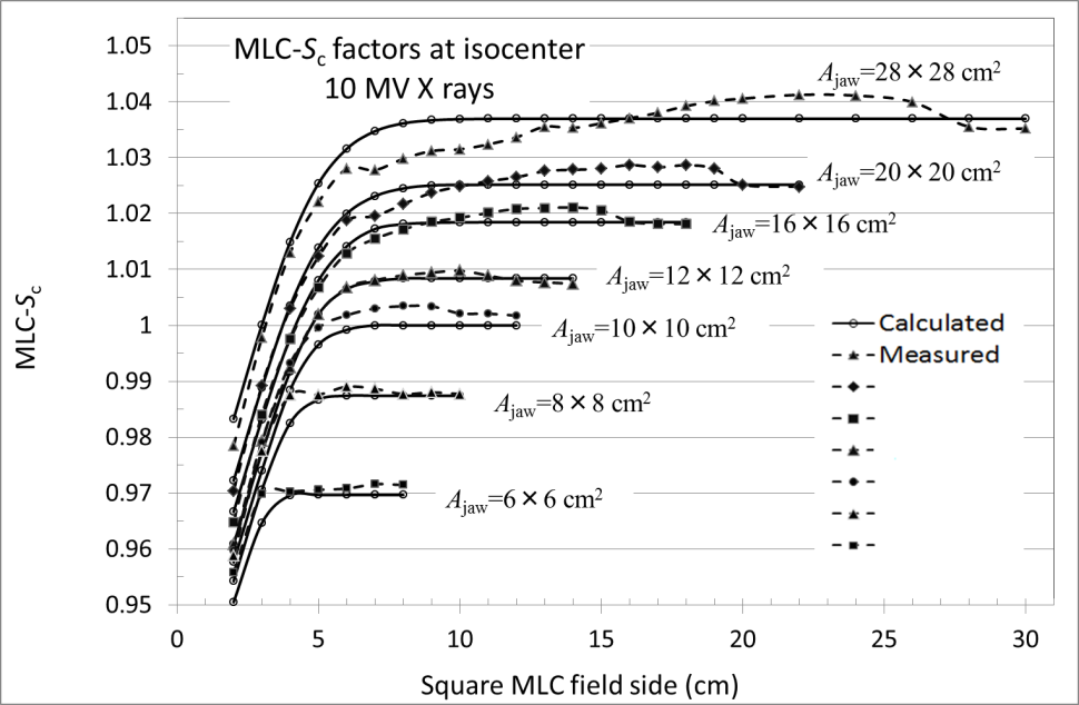
(b) The MLC is simulated by a plate perpendicular to the isocenter axis at the position Z_beam = Z_MLC (= 53.7 cm, which was determined by analyzing the measured MLC-S_c datasets shown in Figure 6 below). We let the plate form the same MLC field as the MLC does on the isocenter plane, corresponding to the MLC effective thicknesses along ray lines emanating from the source (S). This dataset is used to calculate the in-air beam intensity for the open MLC field. It is also used for calculating the dose that the phantom receives from the MLC.

(c) Each of the wedges (15°, 30°, 45° and 60°) and their 0.2 cm acrylic holder are replaced with a plate perpendicular to the isocenter axis at the fixed position Z_beam = Z_wedge (= 42.4 cm), which is the same as the position of the boundary surface of the wedge and its holder. We let the plate form the wedge field as the wedge device does on the isocenter plane, corresponding to the wedge filter and wedge holder thicknesses along ray lines emanating from the source (S). This dataset is used to calculate the dose that the phantom receives from the wedge device and the in-air beam intensity under the wedge-filtered jaw or MLC field.

Figure 4 Drawings of geometrical arrangement for the upper and lower jaws, the MLC and the wedge for (a) the three-dimensional structural devices and for (b) the simplified two-dimensional plate devices.

Figure 5 Schematic diagrams showing how to calculate the OPF_{in_air} factor for a point Q on the isocenter plane when (a) point Q is inside the A_jaw field, and when (b) point Q is outside the A_jaw field (note that, as indicated by the circle mark, the field extends from the A_jaw field edge). It should be noted that the dashed lines are drawn only by taking into account the positions of the lower jaw plates, and that, in like manner, another set of dashed lines should also be utilized by taking into account the positions of the upper jaw plates.

Figure 6 Calculated and measured MLC-S_c datasets obtained at the isocenter (X_beam = 0 cm, Y_beam = 0 cm) as a function of the square MLC field side under each of the square A_jaw fields of 6 × 6-28 × 28 cm².

In-air output factor calculation for open MLC fields
We describe how to calculate the in-air beam intensity for an open MLC field under a given jaw field (without wedge filtration). The calculation is based on the MLC leaf-field output subtraction method [16] at the 15^th ICCR. The details are; Zhu and Bjärngard [17] and Zhu and colleagues [18-20] introduced the 2D Gaussian-source model for the extended radiation source only with a flattening filter to calculate the in-air output factor (S_c) [21, 22] for open jaw or MLC fields. Later, Iwasaki and colleagues [6] proposed the use of this model not only for the flattening filter but also for the X-ray target (or the source (S). It was found that using the two extended radiation sources was effective, even around a zero-area jaw field under conditions of lateral electron disequilibrium. We propose using the two extended radiation sources model to calculate the in-air output factor (OPF_{in_air}) for an open MLC field under a given jaw field by subtracting the in-air output reduction caused by setting the MLC field to the jaw field from the in-air output for the open jaw field (let the in-air output reduction be designated the negative or “black” in-air output). This calculation method can take into account the delicate in-air output variations caused by the MLC leaf curvature and chamfers at the leaf end and the MLC interleaf X-ray leakage.

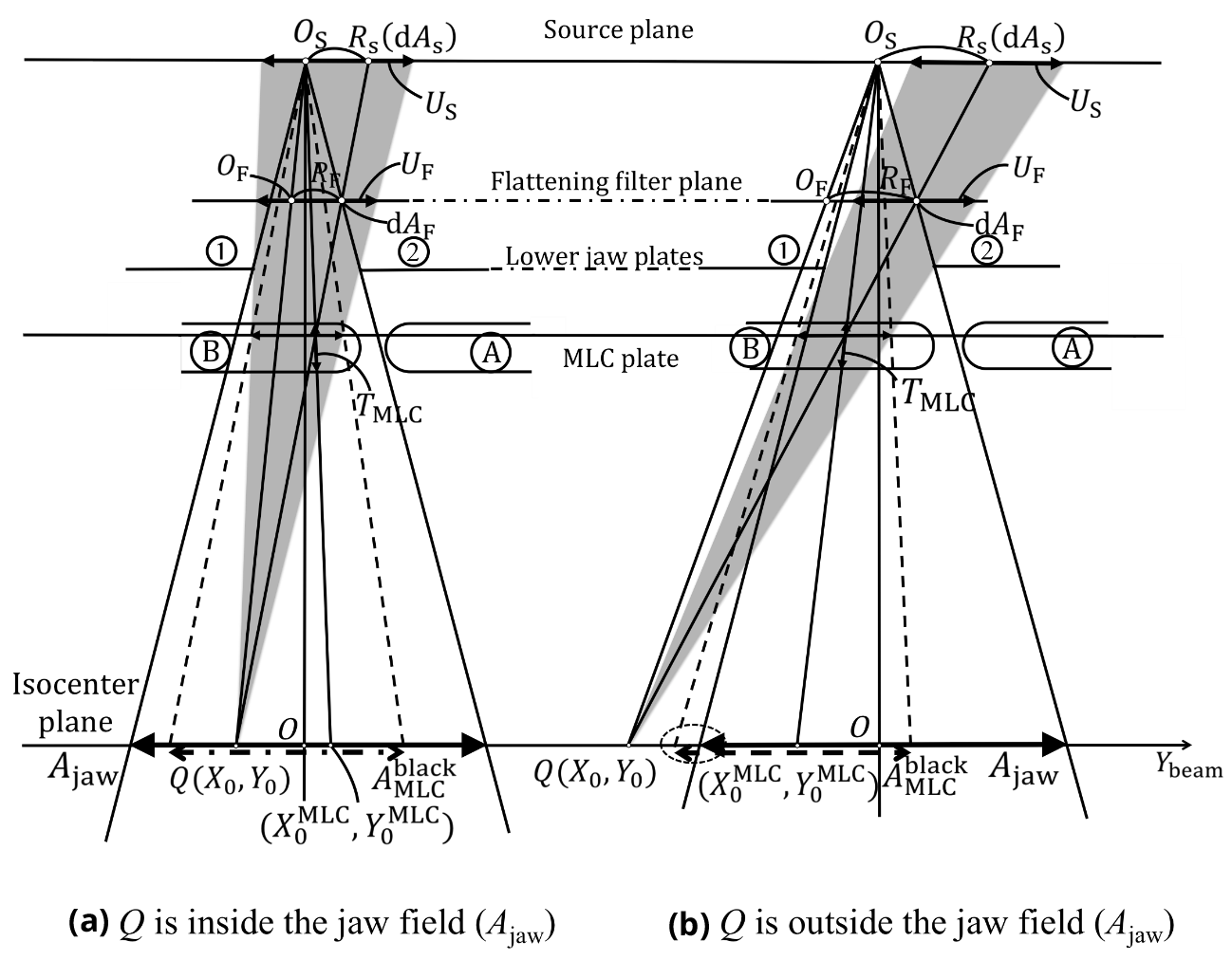
Figure 5 shows the calculation of the OPF_{in_air} factor at a point Q (X₀,Y₀) on the isocenter plane for an open MLC field (A_MLC) under a given jaw field (A_jaw), where Figures 5a, b are drawn for the cases where point Q is inside and outside the A_jaw field, respectively. An extended radiation source exists around point O_S (coinciding with the center of the X-ray target) on the source plate; and another extended radiation source is assumed to exist around point O_F at the intersection of the flattening-filter plate and the ray line connecting points O_S and Q. On the isocenter plane, we introduce a special field called a black MLC field , which is used to evaluate the amount of negative (or black) in-air output, (where the dashed lines in Figures 5a, b are drawn by taking into account the positions of the lower jaw plates (in like manner, another set of dashed lines should also be utilized by taking into account the positions of the upper jaw plates)). It should be emphasized that, if point Q is outside the A_jaw field, the field does not contain point Q. In this case, as indicated by the circle mark in Figure 5b, the field extends beyond the A_jaw field edge. Such an extended region is caused by the treatment of the 2D jaw-collimator plates (the irradiation geometry tells us that, if the real 3D jaw collimator can be utilized, no such large fields can be generated).

We normalize the OPF_{in_air} factor to unity at the isocenter with an open jaw field of A_jaw = 10 × 10 cm² (= 10 × 10_iso), whose center coincides with the isocenter. Then, the OPF_{in_air} factor at point Q (X₀,Y₀) for an open A_MLC field under a given A_jaw field can be calculated as

with , where OCR_source (R₀) is the source off-center ratio [6], obtained by assuming that it is a function of only R₀ for an open infinite A_jaw field (defined as the in-air beam intensity (in water collision kerma) at a point that is R₀ distant from the isocenter to that at the isocenter (that is, OCR_source(0) = 1), where the OCR_source dataset was produced by applying an in-air chamber response function [4] of to an in-air dose dataset measured only at points of Y_beam ≥ 0 on the Y_beam axis). RRF_jaw is the jaw-collimator radiation reflection factor [6], letting RRF_jaw = 1 and RRF_jaw > 1, respectively, inside and outside the A_jaw field. For beams with no MLC device, we obtain by setting A_MLC = ∞ (infinite field) and in equation 23 (see Appendix C for definitions of “off-center jaw-Sc factor”, “MLC-S_c factor” and “jaw-S_c factor”).

First, we formulate [6] H_jaw in equation 23 as

where is the side of the equivalent square field for A_jaw; and a₁, a₂, λ_S and λ_F are constants, where it is assumed that a1 (the monitor-backscatter coefficient) is influenced only by the jaw collimator, which forms the A_jaw field, and not by the MLC or by the wedge. For the present 10-MV X-ray accelerator, we have obtained a₁ = 0.00146 cm^-1, a₂ = 0.0830, λ_S = 0.299 cm and λ_S = 3.097 cm. It can be understood that H_jaw approaches zero as the A_jaw field approaches zero.

Next, we formulate [16] in equation 23 as

where point should be within the region (Figure 5a,b show how point Q, area element dA_S (or dA_F), point O_S and point are related); and γ_MLC is the MLC attenuation factor, evaluated using the beam water collision kerma along the ray line connecting points O_S and as

with , where T_MLC is the MLC effective thickness measured along the ray line connecting points O_S and (it should be noted that we obtain γ_MLC = 1 for T_MLC = 0); (μ_en (E_N)/ρ)water is the mass energy absorption coefficient of water for E_N photons; and expresses the energy fluence spectrum for an open infinite jaw field, as a function of the energy bin (E_N)and the off-axis distance (Figure 7), normalized as .

If T_MLC = 0 for all points on the isocenter plane, we have (that is, no MLC setting for the A_jaw field). Ideally, Y_MLC should be evaluated along the line connecting point Q and dA_S (or dA_F). However, we did not use this procedure, because, along such a line, the spectrum estimation has not yet been established, and calculation of the effective thickness of the MLC is very complicated.

Figure 7 A normalized set of energy fluence spectra (Ψ(E_N, R₀) (N = 1–11)) for 10-MV X-rays (with an accelerating voltage of 10.329 MV), reconstructed at off-axis distances of R₀ = 0, 2.5, 5.0, 7.5, 10.0, 12.5, 15.5, 17.5 and 19.5 cm. The energy bins are E₁ = 0.167 (= E_min), E₂ = 0.627, E₃ = 1.087, E₄ = 1.548, E₅ = 2.008, E₆ = 2.468, E₇ = 3.461, E₈ = 4.987, E₉ = 6.513, E₁₀ = 8.040 and E₁₁ = 9.566 MeV (= E_max) (namely, N_max = 11 and E_mid = 2.698 MeV with ΔE_N = 0.460 MeV for N = 1–6, and with ΔE_N = 1.526 MeV for N = 7–11).

The total in-air energy fluence
For an open infinite jaw field yielding an in-air water collision kerma of OCR_source(R₀) on the isocenter plane (equation 23), the total in-air energy fluence at point (X₀,Y₀) can be evaluated as

with . It should be noted that the denominator of equation 31 expresses the total water collision kerma that the normalized energy fluence spectrum yields at the corresponding point in air. Therefore, the in-air energy fluence related to the normalized energy fluence of Ψ(E_N, R₀) ΔE_N yields the following in-air water collision kerma:

The in-phantom dose calculations described below are carried out using the function. If a wedge filters the open jaw or MLC field, we calculate the in-air water collision kerma variation for each set of primary E_N photons (N = 1 to N_max), depending on the wedge thickness along the corresponding ray line. This is because the in-phantom dose is calculated by using the primary photons emitted from the source (S) and by treating the phantom, the wedge and the MLC as parts of a unified irradiation body.

Calculation of
This section is described mainly by referring to figures 4, 5, 8, and 9, where the 2D wedge and MLC plates are placed at Z_beam = Z_wedge and Z_beam = Z_MLC respectively. We set up the precondition that the 2D wedge and MLC plates hold data regarding the thicknesses (or effective thicknesses) of the 3D wedge and the MLC devices, respectively, measured along the ray lines emanating from the source (S). In the inserted diagram on the right in Figure 8, we let T₀ denote the thickness (or effective thickness) measured along a ray line passing through a point on the wedge or MLC plate and through a point Q(X₀,Y₀) on the isocenter plane, and let α₁ denote the angle between the ray line and the isocenter plane. Then the thickness (or effective thickness) along the line that is parallel to the Z_beam axis and passes through the point can be approximated as T₀ sinα1. Draw an axis r' from a dose calculation point P(X_C, Y_C, Z_C) that passes through the point . Then the thickness (or effective thickness) measured along the r' axis can be approximated as T₀ sinα₁/sinα₂, where α₂ is the angle between the r' axis and the isocenter plane. On the basis of this procedure, the following describes how to handle the 3D wedge and MLC devices.

Figure 8 Diagrams showing how to calculate the thickness (U^L) of the wedge or MLC, measured from the bottom side along the r' axis connecting a dose calculation point P(X_c, Y_c, Z_c) and a point in the wedge or MLC plate, and showing how to calculate the beam water collision kerma at a volume element (ΔV_L) in the wedge or MLC. Let T₀ be the thickness (or effective thickness) of the wedge or MLC, measured along the line connecting the source (S) and a point Q(X₀,Y₀) on the isocenter plane. The inserted diagram on the right is for the case L_max = 5. The diagrams also assist in calculating the beam water collision kermas at an area element (ΔS) on the phantom surface and a volume element (ΔV) in the phantom, in relation to the wedge or MLC setting for the beam.

Figure 9 Diagram showing how to calculate the magnitude of the volume element (ΔV_L) in the L^th section, surrounded by both the ΔL₀ or ΔL'₀ section faces and by the quadrangular pyramid faces determined by (r', θ, Δθ, φ, Δφ) whose apex is located at point P(X_c, Y_c, Z_c). ΔA₀ denotes the area of the pyramid base at point ; perpendicular to the r' axis, and θ'_U denotes the angle between the Z_beam (or Z'_beam axis and the r' axis.

First, we refer to the thickness (or effective thickness) measured from the bottom side along the r' axis using the symbol U^L (L = 1 to L_max). The diagram shows the case when L_max = 5 with equal interval sections ΔL₀ and a residual section ΔL₀ (≤ ΔL'₀) along a line parallel to the Z_beam axis. We estimate the value for U^L as

with

It should be noted that, at least for wedge filters, the calculation for U^L is a close approximation because they are constructed with continuously gentle slope faces against the isocenter plane.

Second, at the point in the Lth section (Figures 8 and 9), we set an imaginary volume element (ΔV_L) that is surrounded both by the ΔL₀ or ΔL'₀ layer faces and by the quadrangular pyramid faces determined by (r', θ, Δθ, φ, Δφ) whose apex is located at point P(X_C, Y_C, Z_C). Let ΔA₀ denote the area of the pyramid base at the point perpendicular to the r' axis; r'_U denotes the distance between points P(X_C, Y_C, Z_C) and and θ'_U denotes the angle between the Z_beam axis (or the Z'_beam axis starting at point P and parallel to the Z_beam axis) and the r' axis. Then the magnitude of (ΔV_L) is given as

with

To calculate the primary and scatter doses from the wedge and MLC bodies, we used ΔL₀ = 0.01 cm and ΔL₀ = 0.1 cm, respectively. To calculate both the primary and scatter doses from the wedge holder, we used ΔL₀ = 0.2 cm (that is, L_max = 1 in Figure 8). The value of T₀ measured along each ray line was obtained by analyzing the manufacturer’s diagrams. However, we assumed that each of the MLC leaves had no driving screw holes (0.33 cm and 0.43 cm in diameter for the 0.5 cm and 1 cm wide leaves, respectively).

Next, we describe the calculation of the beam water collision kermas of (equations 1-3) for a given volume element (ΔV or ΔV_L) or a given area element ΔS within the unified irradiated body (Figure 8). Because the X-ray emission from the flattening filter is very small relative to that from the X-ray target (for the present 10-MV X-ray accelerator, the strength ratio of the extra radiation source to the X-ray target for an infinite A_jaw field is α₂ = 0.0830 (equation 24), we assumed that all X-rays emanate from the source (S).

It has been found that, particularly under MLC field irradiation, the OPF_{in_air} factor (equation 23) determined on the basis of a single point within each ΔV element in the phantom cannot give accurate dose calculation results. This is mainly caused by the nonuniformity of the beam intensities within each ΔV element owing to the use of the MLC. In the following dose calculation procedures, the symbol is used when the beam intensity for each ΔV element in the phantom should be evaluated based on the beam intensity at a single point within each ΔV element. On the other hand, the symbol is used when the in-air beam intensity for each ΔV element in the phantom should be evaluated based on the beam intensities at multiple points within each ΔV element (the details will be described later in equation 47).

Here we classify the wedge irradiation mode using wedge types = 0 to 4, stipulating that wedge type = 0 signifies irradiation with no wedge (that is, open jaw or MLC field irradiations), and wedge types 1, 2, 3 and 4 denote jaw or MLC field irradiations with the use of a 15°, 30°, 45° and 60° wedge, respectively. Under these conditions, the following (a)-(e) describe the evaluation of the beam intensity for a point (L = 1 to L_max) within the MLC or wedge, or for a point (X_U, Y_U, Z_U) on the phantom surface or within the phantom (Figure 8), these points are on a ray line passing through point Q(X₀,Y₀) on the isocenter plane).

(a) For the beam intensity calculation within the MLC device, we set (= 53.7 cm), which is determined by analyzing calculated and measured MLC-Sc datasets (Figure 6). The collision kerma caused by the E_N photons for the ΔV_L element at the point in the Lth section of the MLC plate should be evaluated only under a given A_jaw opening, because the MLC device is placed in close proximity to the jaw collimator; that is, an MLC field of A_MLC = ∞ should be used to evaluate in the following equation. Therefore, the calculation is performed as follows:

where SAD (= 100 cm) is the source–axis distance (or the distance between the source (S) and the isocenter plane); is the effective thickness of the MLC, measured along the corresponding ray line (Figure 8) from the MLC top side to the middle point of the L^th section; and μ_MLC(E_N) is the linear attenuation coefficient of the MLC material for E_N photons.

(b) For the beam intensity calculation within the wedge holder, we set (= 42.4 cm) with L = 1 (= L_max; Figure 8). The collision kerma caused by the E_N photons for the ΔV_L element at the point in the L^th section of the wedge holder should also be evaluated only under a given A_jaw opening (that is, an MLC field of A_MLC = ∞ should be used for in the following equation). Therefore, the calculation is performed as follows:

where T_MLC(X₀,Y₀) is the thickness of the MLC, measured along the corresponding ray line (Figure 8); is the wedge-holder thickness (equation 35) measured along the corresponding ray line, from the wedge-holder top side to the middle point of the L^th section; and μ_{w_hold}(E_N) is the linear attenuation coefficient of the wedge-holder material for the E_N photons. For the case of no MLC in the beam, we should set T_MLC(X₀,Y₀) = 0.

(c) For the beam intensity calculation within the wedge body, we set (= 42.4 cm) with L = 1, 2, ....., L_max (Figure 8). The collision kerma caused by the E_N photons for the ΔV_L element at the point in the L^th section of the wedge body should also be evaluated only under a given A_jaw opening (that is, A_MLC = ∞ should be used for in the following equation). Therefore, the calculation is performed as follows:

where is the wedge-body thickness (equations 34 and 35) measured along the corresponding ray line, from the wedge-body top side to the middle point of the L^th section; and μ_wedge(E_N) is the linear attenuation coefficient of the wedge-body material for the E_N photons. For the case of no MLC in the beam, we should set T_MLC(X₀,Y₀) = 0.

(d) For the beam intensity calculation for the ΔS element at the point (X_U, Y_U, Z_U) on the phantom surface, we should take into account the A_MLC field under a given A_jaw opening. Under the condition that the wedge generally covers the beam, we let the collision kerma for ΔS caused by E_N photons be calculated as follows:

with

where is the field area that the MLC collimator forms inside the A_jaw field on the isocenter plane (that is, ); T_MLC(X₀,Y₀) is the effective thickness of the MLC, measured along the corresponding ray line (note that, for any ray line within the MLC field, we should set T_MLC(X₀,Y₀) = 0); is a factor introduced to make a small correction for the beam intensity calculation by employing , given as a function of both and the wedge type (Appendix D); is a factor introduced to correct for the beam intensity calculation, given as a function of T_MLC(X₀,Y₀) and , finely adjusting the degree of X-ray penetration when passing through the MLC effective thickness of T_MLC(X₀,Y₀) along the corresponding ray line; and T_{w_hold}(X₀,Y₀) and T_wedge(X₀,Y₀) are the thicknesses of the wedge holder and the wedge body, respectively, measured along the ray line (for the case of no wedge device in the beam, we should set T_{w_hold}(X₀, Y₀) = T_wedge(X₀, Y₀) = 0.

(e) To calculate the beam intensity for the ΔV element at the point (X_U, Y_U, Z_U) within the phantom, we should also take into account the A_MLC field under a given A_jaw opening. Here, it should be noted that the ray line passing through the point (X₀, Y₀) on the isocenter plane should also pass through the effective point (Figure 2b) within the ΔV element. It has been found that the same and factors as before should be used to make small corrections also for the beam intensity calculation by employing . Assuming that the wedge generally covers the beam, we let the collision kerma for ΔV caused by the E_N photons are calculated as follows:

where, assuming that the phantom is constructed of water-equivalent media, T_phan(X₀, Y₀) is the effective thickness of the phantom, measured along the ray line from the phantom surface to the point (X_U, Y_U, Z_U) and μ_water(E_N) is the linear attenuation coefficient of water for the E_N photons. For the case of no wedge device in the beam, we should set T_{w_hold}(X₀, Y₀) = T_wedge(X₀, Y₀) = 0. The factor is experimentally constructed as

with

where λ₀ = 1.25 (no units) for the irradiation mode of wedge type = 0 (that is, for open jaw and MLC fields), and λ₀ = 3.50 for the irradiation modes of wedge type = 1-4 (that is, for wedge-filtered jaw and MLC fields). These λ₀ values were obtained by comparing the calculated and measured percentage depth dose (PDD) and off-center ratio (OCR) datasets. This paper uses J_max = 27 as the number of multiple points set within each ΔV element, through which ray lines of J = 1, 2,......, J_max pass (nine points on each of the three planes set perpendicular to the r' axis (Figure 2b); and OPF_J is the OPF_{in_air} factor (equation 23) at the point where the J ray line intersects the isocenter plane (Figure 2b). We have λ_OPF = 0 for for any wedge type. W_OPF expresses the degree of nonuniformity of the incident beam intensity for a given ΔV element, determined by A_jaw, A_MLC and wedge type. It should be noted that, in equation 47, we generally have . It has been found that the work of the factor becomes remarkable as the width of an MLC leaf-blocked section in a jaw field becomes narrow (Figures 10 and 11).

Figure 10 Graphs of the OCR_calc (including its components) and OCR_meas (in points) datasets, with the X_beam value varied with Y_beam = 0 cm on the isocenter plane at a reference depth of Z_R = 5 cm with no wedge used, founded by setting (a) one half-leaf (0.5 cm in width), (b) three consecutive half-leaves (1.5 cm in width) and (c) five consecutive half-leaves (2.5 cm in width) in a jaw field of A_jaw = 10 × 10 cm². 10-MV X-rays, SAD = 100 cm (each reference dose was obtained at Z_R = 5 cm using the open A_jaw field).

Figure 11 Graphs of the OCR_calc (including its components) and OCR_meas (in points) datasets, with the Y_beam value varied and X_beam 1.75 cm on the isocenter plane at a reference depth of Z_R = 10 cm with no wedge used, founded by setting an MLC leaf-blocked section in a jaw field of A_jaw = 10 × 10 cm² with (a) one half-leaf (0.5 cm in width), (b) three consecutive half-leaves (1.5 cm in width) and (c) five consecutive half-leaves (2.5 cm in width). 10-MV X-rays, SAD = 100 cm (each reference dose was obtained at Z_R = 10 cm using the open A_jaw field).

Spectra and dose kernels
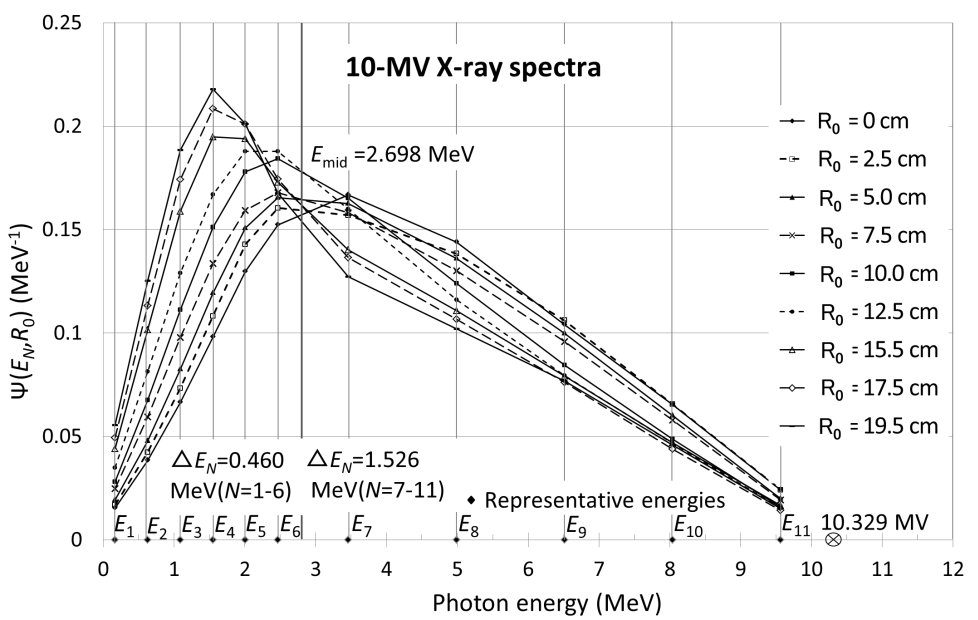
We reconstructed [3, 4] a new set of energy fluence spectra for the accelerator as follows. We measured sets of in-air transmission data at points on the Y_beam axis where Y_beam ≥ 0 using an ionization chamber with an acrylic buildup cap (a factor of f_cap = 0.25 was assumed [4] to account for radiation attenuation and scatter in the buildup cap), in which we used acrylic attenuators of 0–30 cm in thickness and lead attenuators of 0-3 cm in thickness at off-axis distances of R₀ = 0, 2.5, 5.0, 7.5, 10.0, 12.5, 15.5, 17.5 and 19.5 cm. We set a value of 10.329 MV for the accelerating voltage. Using a common set of energy bins for all the off-axis distances, we reconstructed a set of Ψ(E_N, R₀ ) spectra with an accuracy of approximately ±1% for the measured transmission data. The energy bins were E₁ = 0.167 (= E_min), E₂ = 0.627, E₃ = 1.087, E₄ = 1.548, E₅ = 2.008, E₆ = 2.468, E₇ = 3.461, E₈ = 4.987, E₉ = 6.513, E₁₀ = 8.040 and E₁₁ = 9.566 MeV (= E_max) (namely, N_max = 11 and E_mid = 2.698 MeV with ΔE_N = 0.460 MeV for N = 1–6, and with ΔE_N = 1.526 MeV for N = 7–11). Figure 7 shows the reconstructed spectra at R₀ = 0-19.5 cm. The X-ray spectrum becomes softer as the off-axis distance (R₀) increases.

H_1,2 and K_1,2 dose kernels
Primary and scatter dose kernels in water (H_1,2 and K_1,2) for the energy bins of E_N (N = 1 to 11) were produced through use of an Electron Gamma Shower (EGS) Monte Carlo code taking semi-infinite water phantoms (Figure A1). The primary and scatter dose kernels (as shown in Kimura and colleagues [7]) were produced, assuming the density of water to be unity.

Structure of the MLC
The MLC is made of a proprietary tungsten alloy. Accordingly, as an effective approach, we calculated the in-air output factor (OPF_{in_air}) for an open MLC field using equation 23 by assuming that the MLC was composed of tungsten atoms; however, its density was different from that of pure tungsten metal. We let the ratio of the mass density of the MLC material to that of the pure tungsten material be ρ_{MLC_factor} = 0.897 This ratio was obtained by comparing calculated and measured MLC-S_c datasets (Figure 6), which we calculated by setting a virtual 2D MLC plate at a distance of Z_MLC = 53.7 cm above the isocenter plane (Figure 4). On the whole, these numerical values gave the most accurate results for the MLC-S_c factor.

The MLC device is composed of sixty pairs of leaves. Let N^leaf denote the leaf number. At N^leaf = 1 and N^leaf = 60, each of the leaves forms a special shadow field 1.4 cm wide on the isocenter plane. At N^leaf = 2-10 and N^leaf = 51-59, each of the leaves forms a shadow field 1 cm wide, called a “full leaf” or “type 0.” At N^leaf = 11-50 forms a shadow field 0.5 cm wide, called a “half leaf.” The half leaves are classified into two types, type 1 and type 2, and these types are arrayed alternately. The full and half leaves have [23] a staple, a hook, a curved end, stepped sides and chamfers at both corners of the curved end so that these leaves can be moved to create an irregular field shape.

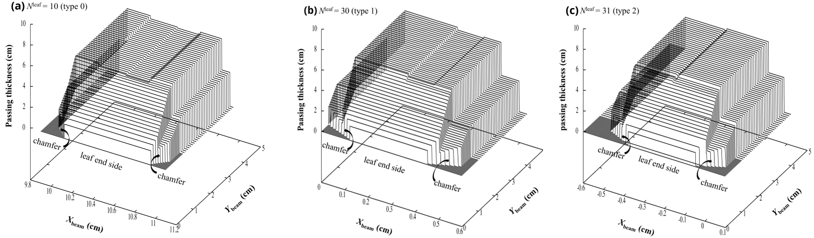
We analyzed the fine 3D structure of the full and half leaves as per the manufacturer’s information. When the full and half leaves are consecutively arrayed, the isocenter-axis components of the MLC effective thicknesses calculated along the ray lines are separated into seven or eight sections, respectively, in the direction of the X_beam-axis (excluding the region around each curved end and ignoring the presence of the driving screw holes). Figure 12 illustrates the sectional widths measured on the isocenter plane for leaves of (a) type 0 (full), (b) type 1 (half) and (c) type 2 (half). The width of the region overlapped with the neighboring leaf is 0.067 cm; accordingly, each type has an actual width of 0.567 or 1.067 cm. The data in brackets give the isocenter-axis components. Figure 13 illustrates the 3D shapes of the isocenter-axis components for a single full or half leaf: (a) full leaf (type 0; using N^leaf = 10), (b) half leaf (type 1; using N^leaf = 30) and (c) half leaf (type 2; using N^leaf = 31). Note that the diagrams are drawn by setting the position of each leaf end at Y_beam = 0 cm.

Figure 12 Sectional widths measured on the isocenter plane for leaves of (a) type 0 (full), (b) type 1 (half) and (c) type 2 (half). Each type has an actual width of 0.567 or 1.067 cm. Data in brackets show the isocenter-axis components of the MLC effective thicknesses measured along ray lines when the full or half leaves are continuously arrayed, excluding the region around each curved end and ignoring the presence of the driving screw hole.

Figure 13 The 3D shapes of the isocenter-axis components of the MLC effective thicknesses calculated along ray lines, as a function of X_beam and Y_beam, for a single full or half leaf whose leaf end point is at Y_beam = 0 cm (ignoring the presence of the driving screw hole): (a) for the full leaf (type 0; using N^leaf = 10), (b) for the half leaf (type 1; using N^leaf = 30) and (c) for the half leaf (type 2; using N^leaf = 31).

MLC-S_c calculation
Using equation 23, we calculated the in-air output factor (OPFin_air) under a given set of A_MLC and A_jaw fields along each center line of the seven or eight stripes using its sectional width (Figure 12) for each of the full or half MLC leaves. However, for N^leaf = 1 and 60 we assumed that each leaf had an infinite width, repeating the eight-striped pattern of the full leaf (to take into account the overrun area, as indicated by the circle in Figure 5b, when the X_beam-axis side edge of the A_jaw field is nearly equal to ±20 cm). Moreover, to effectively calculate OPF_{in_air} near the leaf end, we used a series of ΔT^leaf steps on the middle line of each stripe, starting at the leaf end, as follows:

for i = 1, 2, 3, ......., where we let and . Then, we have and (the step increases slowly at small and large values of i). For the experimental studies, we used and .

Figure 6 shows the calculated and measured MLC-S_c datasets that were obtained at the isocenter (X₀ = Y₀ = 0 cm) as a function of the square A_MLC field side under each of the square A_jaw fields of 6 × 6 to 28 × 28 cm² in size (equation C2 in Appendix C), letting both A_MLC and A_jaw fields be symmetric with respect to the X_beam and Y_beam axes, and letting the other pairs of A and B MLC leaves be closed at Y_beam = 0 cm. The measurement was performed using a cylindrical mini-phantom [24] with a 0.6 cm³ chamber (PTW 30006 Waterproof Farmer Chamber, Radiation Products Design, Inc. Albertville MN, USA) in free air. It can be seen that the measurement, having small waveforms for each of the A_jaw fields, seems to be influenced to a certain degree by scattered radiation from the MLC leaves.

The mean absolute deviation of the calculations is 0.21% (the minimum is -0.71% and the maximum is 0.68%). The MLC-S_c factor depends largely on the A_jaw field; however, under a given A_jaw field, the MLC-S_c factor rapidly decreases from a certain A_MLC field size as the A_MLC field becomes smaller. It should be noted that, when the positions of the pairs of closed leaves are set at Y_beam = ±30 cm, the mean absolute deviation of the calculations is 0.22% (the minimum is -0.77% and the maximum is 0.67%).Therefore, it is clear that the in-air output factor (OPF_{in_air}) is influenced by the shapes of the MLC leaf structures. This is because the value of calculated by setting the positions of the closed leaves at Y_beam = ±30 cm is greater than that calculated with Y_beam = 0 cm.

Structure of the wedge filters
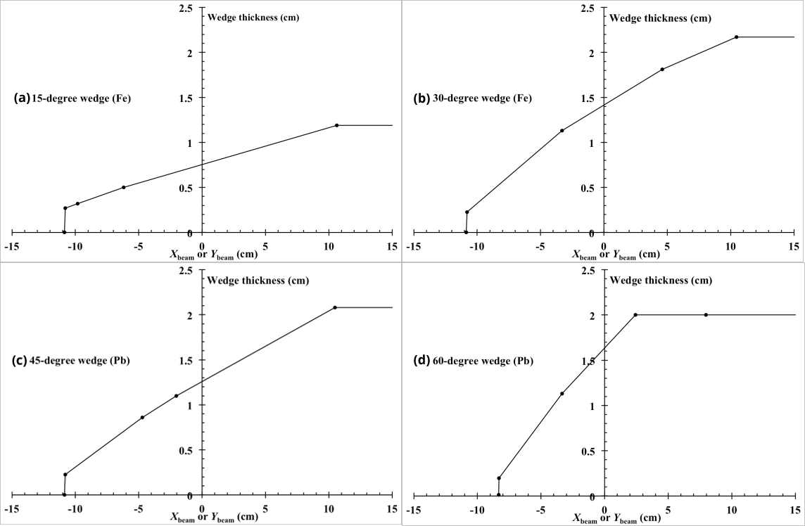
The 15° and 30° wedge filters are made of proprietary iron alloys, and the 45° and 60° wedge filters are made of proprietary lead alloys. Accordingly, to effectively calculate the wedge-filtered dose, we introduced a factor, called ρ_{wedge_factor}, giving the ratio of the mass density of the wedge material to that of pure iron or lead (assuming, to a first approximation, that the wedge material is composed of iron or lead, though its density is different from the density of pure iron or lead) for each of the four wedges. We set ρ_{wedge_factor} = 0.900 for the 15° wedge; ρ_{wedge_factor} = 0.915 for the 30° wedge; ρ_{wedge_factor} = 0.955 for the 45° wedge; and ρ_{wedge_factor} = 0.930 for the 60° wedge. These factors were obtained by comparing calculated and measured PDD and OCR datasets.

Each wedge body is attached to a 0.2 cm thick acrylic plate. Figure 14 shows cross-sectional body views of the wedges. The vertical axis shows the isocenter-axis components of the wedge thickness measured along ray lines, as a function of X_beam or Y_beam on the isocenter plane. Each view forms a polygonal structure with corners marked by dots.

Figure 14 Cross-sectional body views of (a) the 15° wedge (steel alloy), (b) the 30° wedge (steel alloy), (c) the 45° wedge (lead alloy) and (d) the 60° wedge (lead alloy). The vertical axis shows the isocenter-axis components of the wedge thickness measured along ray lines, as a function of X_beam or Y_beam.

Calculation of PDD and OCR
The dose calculations in water phantoms described below were performed by setting the density of water to 0.990 g/cm³ to obtain the most accurate calculation results (this value is approximately 0.65% less than that at room temperature). We calculated the dose at a point P(X_c, Y_c, Z_c) in a water phantom, using a polar coordinate system (r', Φ, θ) derived from the (x_v, y_v, z_v) coordinate system (Figure 2). Using the procedures described in Appendix B for setting steps of (Δr', ΔΦ, Δθ) and for setting the effective point for each volume element ΔV on the r'-axis, the dose calculation ability was assessed with PDD and OCR datasets that were measured in water phantoms using a 0.125 cm³ ionization chamber (dimension of sensitive volume: radius 2.75 mm, length 6.5 mm; PTW 31002, Radiation Products Design, Inc.), setting the effective center of the chamber to coincide with each measuring point.

Setting the source–surface distance (SSD) to be 100 cm (equal to the source–axis distance (SAD)), we let the PDD be defined along the isocenter axis (X_beam = Y_beam = 0 cm) as:

where D₁ in the numerator is the dose at a phantom at depth Z on the isocenter axis for an MLC field (A_MLC) under a jaw field (A_jaw) with no wedge used (wedge type = 0) or with one of the four wedges (wedge type = 1-4, also indicating its insertion direction); and D₁ in the denominator is the reference dose at a phantom at a reference depth of Z_R = 10 cm on the isocenter axis under a reference jaw field of with no MLC (namely, , an infinite field) and with no wedge (wedge type_R = 0), where the symbol is used below as the reference dose.

Next, setting the source–chamber distance (SCD) to be 100 cm (= SAD), we let the OCR be defined at a point (X_beam, Y_beam) on the isocenter plane (Z_beam = 0 cm) as:

where D₂ in the numerator is the dose at a point (X_beam, Y_beam) on the isocenter plane at a reference depth of Z_R on the isocenter axis for an MLC field (A_MLC) under a jaw field (A_jaw) with no wedge filter (wedge type = 0) or with one of the four wedges (wedge type = 1-4) also indicating its insertion direction); and D₂ in the denominator is the reference dose at the isocenter point on the isocenter plane at the reference depth (Z_R) under a reference jaw field of with no MLC (namely, and with no wedge (wedge type_R = 0), where the symbol is used below as the reference dose.

According to the section of Dose calculation principle, each of D₁ and D₂ in equations 52 and 53 is typically composed of the nine dose components or the three dose components (D_prim, D_scat and D_cont).

Experimental studies and discussionTop

The PDD and OCR datasets in the water phantoms were calculated and measured, where the square A_MLC and A_jaw fields used below were all symmetric with respect to the X_beam and Y_beam axes. It should be noted that, for any given square A_MLC field, the MLC leaves not taking part in forming the open A_MLC field were intentionally closed at Y_beam = 0 cm, and that each of the measured PDD or OCR datasets (drawn in dots in the figures below), producing the ratio of the dose relative to the reference dose, had a relative error of approximately ±0.7% because each measurement of D₁ and D₂ at a fixed point had a relative error of approximately ±0.5%.

PDD datasets
The calculated and measured PDD (PDD_calc and PDD_meas) datasets, given as a function of the depth (Z) of a phantom on the isocenter axis under each irradiation condition, are shown below. Let the PDD_calc components corresponding to the nine dose components mentioned above be expressed as:

Then we have:

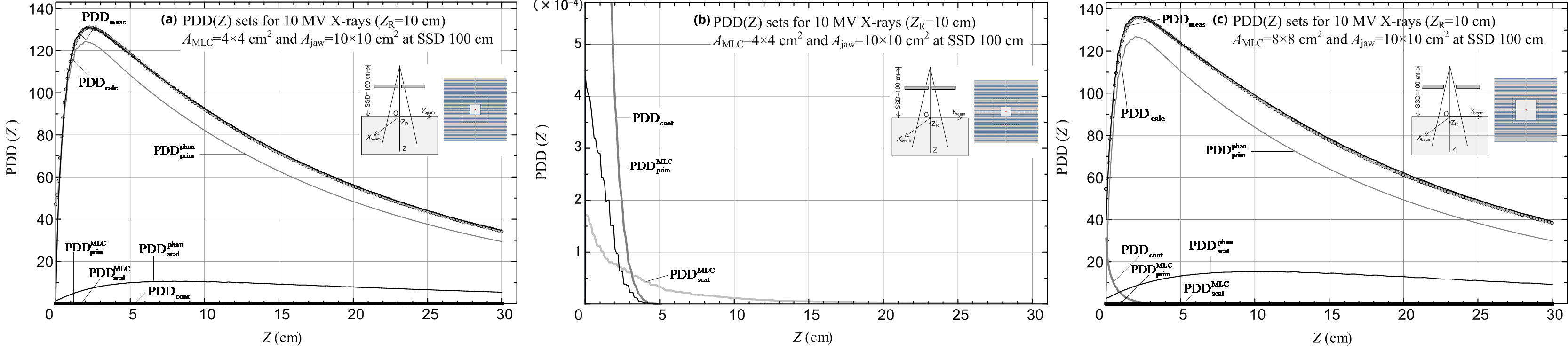
First, PDD(Z) datasets with no wedge used were calculated and measured for combinations of square A_MLC and A_jaw fields. We set MLC fields of A_MLC = 4 × 4-10 × 10 cm² for a jaw field of A_jaw = 10 × 10 cm²; we set MLC fields of A_MLC = 4 × 4-15 × 15 cm² for a jaw field of A_jaw = 15 × 15 cm²; and we set MLC fields of A_MLC = 4 × 4-20 × 20 cm² for a jaw field of A_jaw = 20 × 20 cm². Figures 15a-c show the PDD_calc (including its components) and PDD_meas datasets: diagram (a) is for a combination of A_MLC = 4 × 4 cm² and A_jaw = 10 × 10 cm² (details of the lower dose components are shown in diagram (b)); and diagram (c) is for a combination of A_MLC = 8 × 8 cm² and A_jaw = 10 × 10 cm² fields. It can be seen that (a) each of the primary and scatter doses from the MLC can be ignored; (b) the electron contamination dose decreases as the A_MLC field decreases for a given A_jaw field; and (c) the calculated data at depths greater than around 20 cm are approximately 1–2% greater than the corresponding measured data (this paper does not analyze further why such large deviations were produced); and (d) and PDD_cont = 0 at depths greater than approximately 5.8 cm. Results with almost the same calculation accuracy were also obtained for the other combinations of A_MLC and A_jaw fields.

Figure 15 Graphs of the PDD_calc (including its components) and PDD_meas (in points) datasets in water with no wedge for (a) A_MLC = 4 × 4 cm² and A_jaw = 10 × 10 cm² (details of the lower dose region are shown in (b)) and for (c) A_MLC = 8 × 8 cm² and A_jaw = 10 × 10 cm². 10-MV X-rays, SSD = 100 cm (each reference dose was obtained at Z_R = 10 cm using the open A_jaw field).

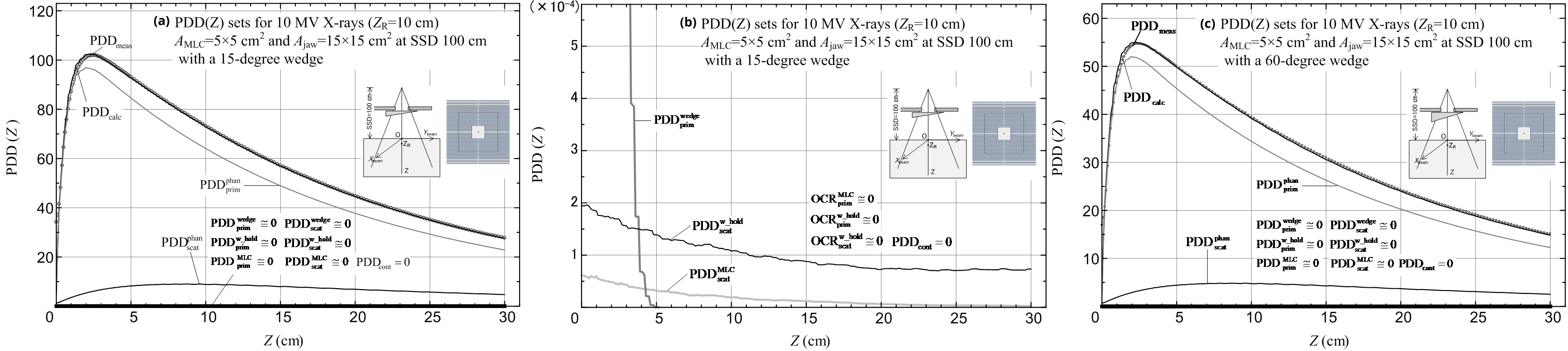
Second, PDD(Z) datasets using the 15°, 30°, 45° and 60° wedges in the direction of the Y_beam axis were calculated and measured for combinations of square A_MLC and A_jaw fields as follows: we set A_MLC = 4 × 4 - 10 × 10 cm² for a jaw field of A_jaw = 10 × 10 cm²; we set A_MLC = 4 × 4-15 × 15 cm² for a jaw field of A_jaw = 15 × 15 cm²; and we set A_MLC = 4 × 4-20 × 20cm² for a jaw field of A_jaw = 20 × 20 cm² (excluding the case where the 60° wedge is used). Figures 16a-c show the PDD_calc (including its components) and PDD_meas datasets for a combination of A_MLC = 5 × 5 cm² and A_jaw = 15 × 15 cm² fields: diagram (a) is for the 15° wedge (details of the lower dose components are shown in diagram (b)); and diagram (c) is for the 60° wedge. It can be seen that the electron contamination dose virtually vanishes with the use of each of the wedges (namely, PDD_cont = 0), and that each of the primary and scatter doses from the wedge and MLC can be ignored (namely, where at depths greater than approximately 5.6 cm). The calculation results in the buildup region are relatively poor (Figure 16a shows deviations = -28.2% (Z = 0.008 cm) to 6.8% (Z = 0.8 cm), and Figure 16c shows deviations = -80.7% (Z = 0.008 cm) to 8.2% (Z = 0.8 cm); this paper does not analyze further why such large deviations were produced), although the calculation results at depths beyond the buildup region are relatively accurate (Figure 16a shows deviations = -0.6% (Z = 10.2 cm) to 0.3% (Z = 2.6 cm), and Figure 16c shows deviations = -2% (Z = 30 cm) to 0.5% (Z = 2.5 cm). Results with almost the same calculation accuracy were also obtained for the other PDD datasets.

Figure 16 Graphs of the PDD_calc (including its components) and PDDmeas (in points) datasets for A_MLC = 5 × 5 cm² and A_jaw = 15 × 15 cm² with the use of (a) a 15° wedge (details of the lower dose region are shown in (b)) and (c) a 60° wedge (each in the direction of the Y_beam axis). 10-MV X-rays, SSD = 100 cm (each reference dose was obtained at Z_R = 10 cm using the open A_jaw field).

OCR datasets
This section presents details of the calculated and measured OCR (OCR_calc and OCR_meas) datasets, with the Y_beam value varied and X_beam kept constant, or with the X_beam value varied and Y_beam kept constant, on the isocenter plane at the reference depth (Z_R) under each irradiation condition. Let the OCR_calc components corresponding to the nine dose components mentioned above be expressed as:

Then we have:

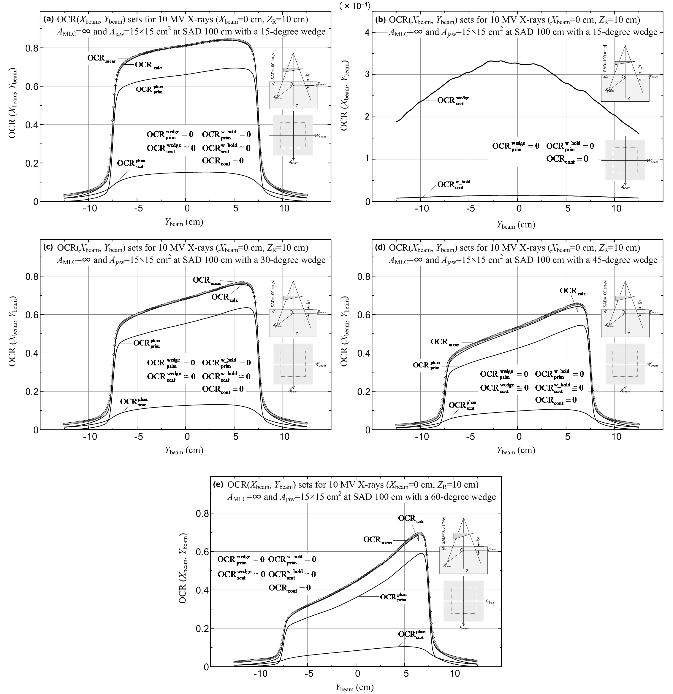
First, we calculated and measured the OCR(X_beam, Y_beam) datasets, with the Y_beam value varied and X_beam = 0 cm on the isocenter plane at a reference depth of Z_R = 10 cm, setting each of the four wedges in the direction of the Y_beam axis and with no MLC (A_MLC = ∞). When using the 15°, 30° and 45° wedges, we set square jaw fields of A_jaw = 5 × 5 - 20 × 20 cm². When using the 60° wedge, we set square jaw fields of A_jaw = 5 × 5 - 15 × 15 cm². Figures 17a-e show the OCR_calc (including its components) and OCR_meas datasets for a jaw field of A_jaw = 15 × 15 cm²: diagram (a) is for the 15° wedge (details of the lower dose components are shown in diagram (b)); diagram (c) is for the 30° wedge; diagram (d) is for the 45° wedge; and diagram (e) is for the 60° wedge. We obtain and at points around Y_beam = 0 cm. For all the calculation points, we obtain OCR_cont = 0, and (because the contaminant electrons and the secondary electrons from the wedge device are all shielded by the wedge and the 10 cm of water). In general, both the OCR_calc and OCR_meas datasets were in good agreement (with deviations of -0.03 to 0.09% at points around Y_beam = 0 cm), except in the case of Figure 17d with a relatively large deviation of -1.5% at points around Y_beam = 0 cm (this paper does not analyze further why such large deviations were produced). Results with almost the same calculation accuracy were also obtained for the other OCR datasets.

Figure 17 Graphs of the OCR_calc (including its components) and OCR_meas (in points) datasets, with the Y_beam value varied and X_beam = 0 cm on the isocenter plane at a reference depth of Z_R = 10 cm , for A_jaw = 15 × 15 cm² with no MLC and the following wedges set in the direction of the Y_beam axis: (a) a 15° wedge (details of the lower dose region are shown in (b)); (c) a 30° wedge; (d) a 45° wedge; and (e) a 60° wedge. 10-MV X-rays, SAD = 100 cm (each reference dose was obtained at Z_R = 10 cm using the open A_jaw field).

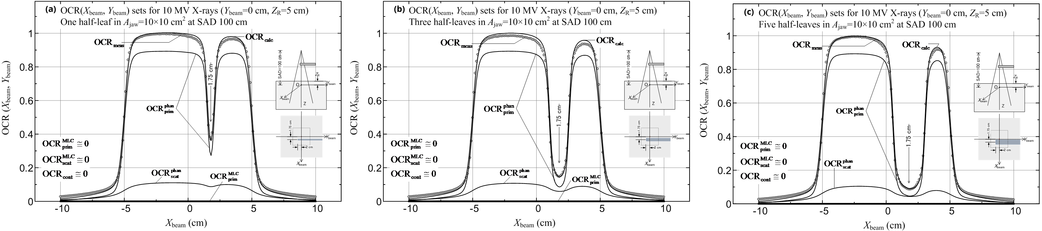
Next, we calculated and measured the OCR(X_beam, Y_beam) datasets, with the X_beam value varied and Y_beam = 0 cm on the isocenter plane at each reference depth of Z_R = 2.5, 5 and 10 cm with no wedge used by setting each of the following three MLC leaf-blocked sections within a jaw field of A_jaw = 10 × 10 cm². Figures 10a-c show the OCR_calc (including its components) and OCR_meas datasets for Z_R = 5 cm with the use of MLC leaf-blocked sections: diagram (a) is for one half-leaf (0.5 cm in width); diagram (b) is for three consecutive half-leaves (1.5 cm in width); and diagram (c) is for five consecutive half-leaves (2.5 cm in width). For all the calculation points, we obtained OCR_cont ≅ 0 (because the contaminant electrons are practically shielded by the 5 cm thick water layer), and also obtained and . It can be seen that the OCR_meas data behind the MLC leaf-blocked section by the one half-leaf (Figure 10a) are slightly greater (2.5%) than the OCR_calc data because the chamber readings are somewhat influenced by higher doses in the non-leaf-blocked regions, and that, in the non-leaf-blocked regions, the OCR_calc data are around 2% greater than the OCR_meas data (these large deviations may be due to the assumption that OCR_source is a function of only the off-axis distance (R₀); in fact, the basic OCR_source dataset was produced based only on in-air dose data measured at points where Y_beam ≥ 0 on the Y_beam axis). Almost the same calculation accuracy was also observed for the other datasets. It should be emphasized that the work of the factor (equation 47) becomes remarkable as the width of an MLC leaf-blocked section in a jaw field becomes narrow. The same statement can also be referred to the cases of Figures 11a-c described in the next place.

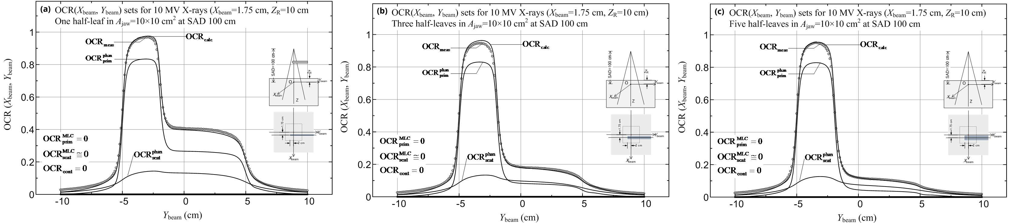
Next, we calculated and measured the OCR(X_beam, Y_beam) datasets with the Y_beam value varied and X_beam = 1.75 cm on the isocenter plane at each reference depth of Z_R = 2.5, 5 and 10 cm with no wedge used by setting each of the following three MLC leaf-blocked sections in a jaw field of A_jaw = 10 × 10 cm². Figures 11a-c show the OCR_calc (including its components) and OCR_meas datasets for X_beam = 1.75 cm and Z_R = 10 cm: diagram (a) is for one half-leaf (0.5 cm); diagram (b) is for three consecutive half-leaves (1.5 cm); and diagram (c) is for five consecutive half-leaves (2.5 cm). For all the calculation points, we obtained OCR_cont = 0 (because the contaminant electrons are practically all shielded by the 10 cm of water), and also obtained and . The OCR_meas data behind the MLC leaf-blocked section by the one half-leaf (Figure 11a) are slightly greater (3.5%) than the OCR_calc data because the chamber readings are also influenced by higher doses in the non-leaf-blocked regions. In Figure 11b, the OCR_calc data in the non-leaf-blocked region are around 2% greater than the OCR_meas data (this paper does not analyze further why such large deviations were produced). Figures 11a-c reveal that certain amounts of radiation leak at points which are behind the MLC leaf-blocked sections but within the jaw field. Results with almost the same calculation accuracy were also observed for the other datasets.

Next, we calculated and measured the OCR(X_beam, Y_beam) datasets, with the Y_beam value varied and X_beam = 0, 1.25 and 3.75 cm on the isocenter plane at each reference depth of Z_R = 2.5, 5 and 10 cm with the use of each of the four wedges in the direction of the Y_beam axis. For each of the 15°, 30° and 45° wedges, we set an MLC field of A_MLC = 5 × 5 cm² for the jaw fields of A_jaw = 10 × 10, 15 × 15 and 20 × 20 cm². For the use of the 60° wedge, we set an MLC field of A_MLC = 5 × 5 cm² for the jaw fields of A_jaw = 10 × 10 and 15 × 15 cm². Figures 18a-e show the OCR_calc (including its components) and OCR_meas datasets for X_beam = 0 cm and Z_R = 10 cm with a combination of A_MLC = 5 × 5 cm² and A_jaw = 15 × 15 cm² fields: diagram (a) is for the 15° wedge (details of the lower dose region are shown in diagram (b)); diagram (c) is for the 30° wedge; diagram (d) is for the 45° wedge; and diagram (e) is for the 60° wedge. For all the calculation points, we obtained OCR_cont = 0, , and (because the contaminant electrons and the secondary electrons from the MLC and wedge devices cannot reach each of the calculation points), and also obtained and . We obtained at points around Y_beam = 0. Figures 18a, c-e show that the deviations of the OCR_calc data at Y_beam = 0 cm are -0.8%, -1.8%, -1.1% and -1.8%, respectively (these deviations may be caused by the inaccurate estimates of ρ_{wedge_factor} given for the wedges under the given OCR_source distribution), and that certain amounts of X-rays leak at points which are outside the MLC field but within the jaw field. Similar results were also observed in other irradiation cases, as described below. Results with almost the same calculation accuracy were also obtained for the other OCR datasets.

Figure 18 Graphs of the OCR_calc (including its components) and OCR_meas (in points) datasets, with the Y_beam value varied and X_beam = 0 cm on the isocenter plane at a reference depth of Z_R = 10 cm, for A_MLC = 5 × 5 cm² and A_jaw = 15 × 15 cm² with the use of (a) a 15° wedge, (b) details of the lower dose region, (c) a 30° wedge, (d) a 45° wedge and (e) a 60° wedge (each in the direction of the Y_beam axis). 10-MV X-rays, SAD = 100 cm (each reference dose was obtained at Z_R = 10 cm using the open A_jaw field).

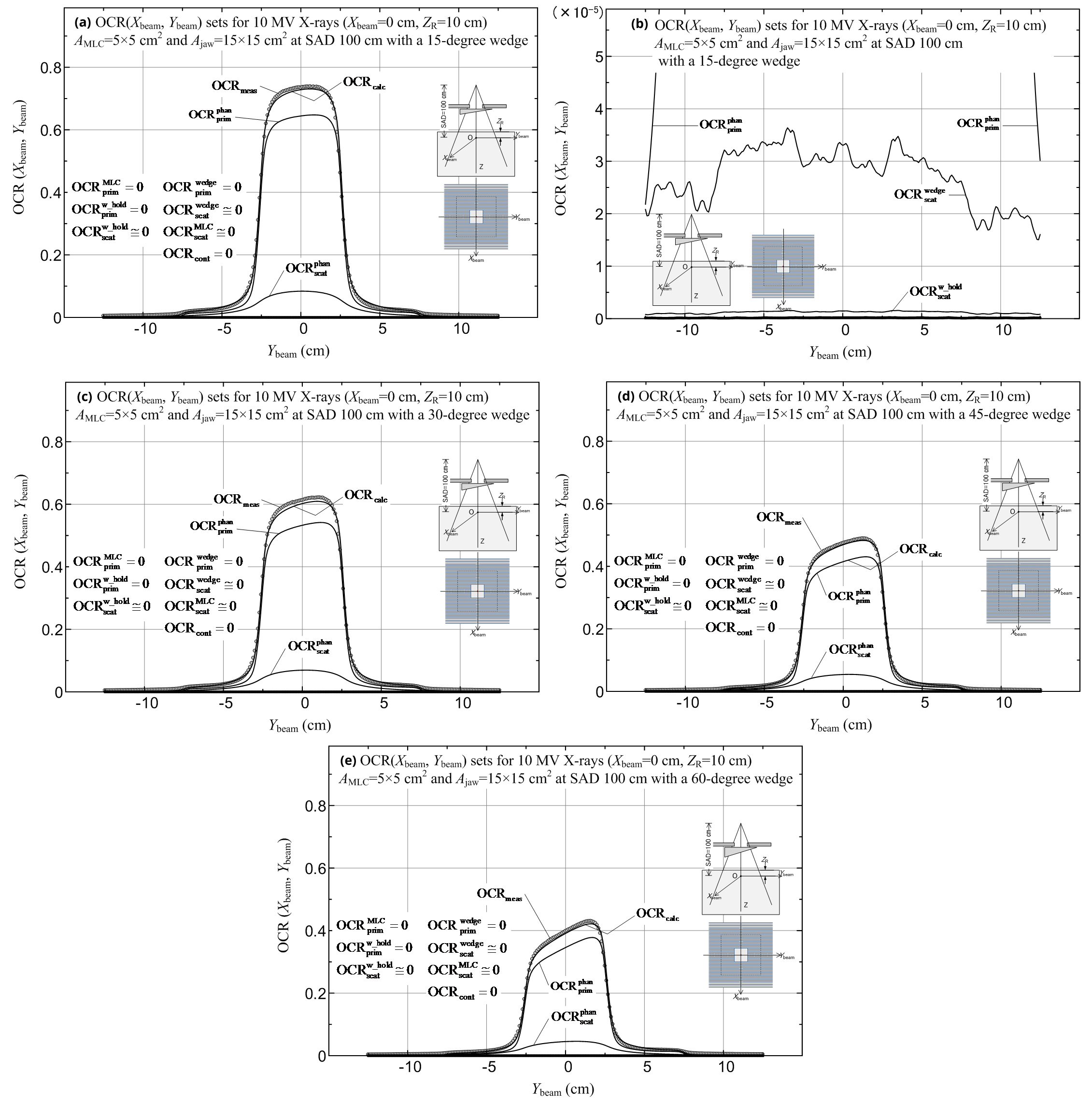
Next, we calculated and measured the OCR(X_beam, Y_beam) datasets, with the Y_beam value varied and X_beam = 0, 1.25 and 3.75 cm on the isocenter plane at each reference depth of Z_R = 2.5, 5 and 10 cm using each of the four wedges in the direction of the Y_beam. When using the 15°, 30° and 45° wedges, we set square jaw fields of A_jaw = 5 × 5 - 20 × 20 cm². When using the 60° wedge, we set square jaw fields of A_jaw = 5 × 5 - 15 × 15 cm². Figures 19a-c show the OCR_calc (including its components) and OCR_meas datasets for Z_R = 10 cm, with the use of the 45° wedge for a combination of A_MLC = 5 × 5 cm² and A_jaw = 15 × 15 cm² fields: diagram (a) is for X_beam = 0 cm; diagram (b) is for X_beam = 1.25 cm; and diagram (c) is for X_beam = 3.75 cm. For all the calculation points, we obtained OCR_cont = 0 (because the contaminant electrons are all shielded by the wedge and the 10 cm thick water layer), and also obtained , and (because the secondary electrons from the MLC and wedge devices cannot reach each of the calculation points). We obtained , and at points around Y_beam = 0 cm. The OCR_calc deviations at Y_beam = 0 cm are -1.1% in Figure 19a and -1.9% in Figure 19b (these deviations may also be caused by the inaccurate estimate of ρ_{wedge_factor} given for the wedge under the given OCR_source distribution). Figure 19c similarly shows the results for X_beam = 3.75 cm outside the A_MLC field, illustrating the sharp changes in dose distribution near the point of Y_beam = 0 cm (due to the large X-ray leakage from the closed parts, where the pairs of A- and B-MLC leaves are just closed). It also demonstrates that the OCR_meas data are smaller than the OCR_calc data at points around Y_beam = 0 cm, because the measurements by the chamber reflect the lower doses in the MLC-shielded region. Figures 19a-c show that certain amounts of X-rays leak at points which are outside the MLC field but within the jaw field. Almost the same calculation accuracy was also observed for the other OCR datasets.

Figure 19 Graphs of the OCR_calc (including its components) and OCR_meas (in points) datasets, with the Y_beam value varied and (a) X_beam = 0 cm (b) X_beam = 1.25 cm and (c) X_beam = 3.75 cm on the isocenter plane at a reference depth of Z_R = 10 cm, with the use of a 45° wedge in the direction of the Y_beam axis for A_MLC = 5 × 5 cm² and A_jaw = 15 × 15 cm². 10-MV X-rays, SAD = 100 cm (each reference dose was obtained at Z_R = 10 cm using the open A_jaw field).

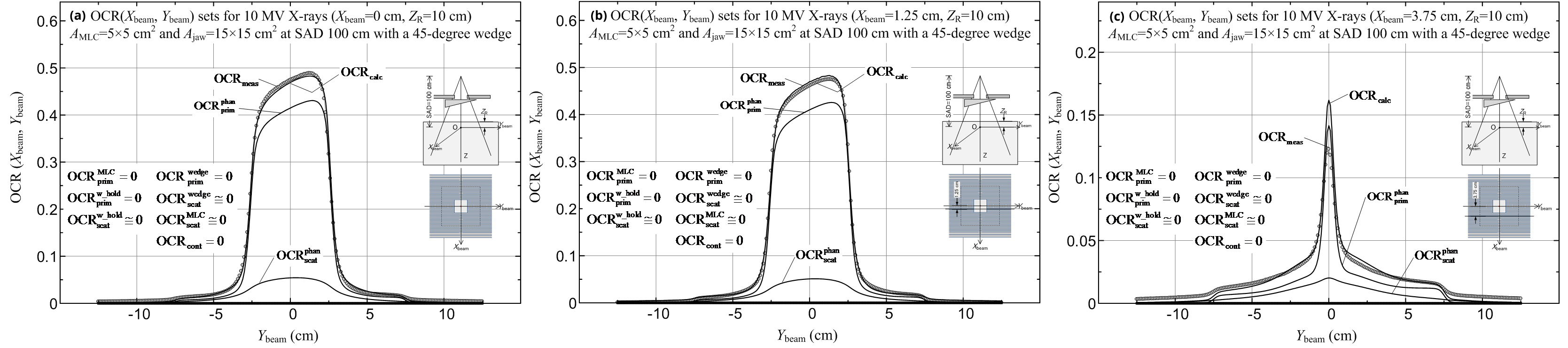
Finally, we calculated and measured the OCR(X_beam, Y_beam) datasets, with the X_beam value varied and Y_beam = 0, -1.25 and -3.75 cm on the isocenter plane at each reference depth of Z_R = 2.5, 5 and 10 cm, using the four wedges in the direction of the X_beam axis. When using the 15°, 30° and 45° wedges, we set square jaw fields of A_jaw = 5 × 5 - 20 × 20 cm² for an MLC field of A_MLC = 5 × 5 cm². When using the 60° wedge, we set square jaw fields of A_jaw = 5 × 5 - 15 × 15 cm² for an MLC field of A_MLC = 5 × 5 cm². Figures 20a-c show the OCR_calc (including its components) and OCR_meas datasets for Z_R = 10 cm with the use of the 45° wedge for a combination of A_MLC = 5 × 5 cm² and A_jaw = 15 × 15 cm² fields: diagram (a) is for Y_beam = 0 cm; diagram (b) is for Y_beam = -1.25 cm; and diagram (c) is for Y_beam = -3.75 cm. These OCR_calc and OCR_meas results clearly indicate variations in X-ray beam attenuation along the direction of wedge insertion. With respect to each of the diagrams, we obtained OCR_cont = 0, , and for all the calculation points (because the contaminant electrons and the secondary electrons from the MLC and wedge devices cannot reach each of the calculation points); and we obtained , and near the point of X_beam = 0 cm Figure 20a shows waveform dose distributions in the left- and right-hand regions that are outside the MLC field but within the jaw field, where the pairs of A- and B-MLC leaves are just closed. In the waveform dose distributions, the OCR_meas data are much smaller than the OCR_calc data because the measurements by the chamber of finite size reflect the lower doses in the MLC-shielded region. There are relatively large deviations in OCR_calc resulting from the measurement (OCR_meas) at X_beam = 0 cm; Figure 20a shows -1.1%, and Figure 20b shows -1.7% (these deviations may also be caused by the inaccurate magnitude of ρ_{wedge_factor} given for the wedge under the given OCR_source distribution). Figure 20c shows the OCR datasets outside the A_MLC field, illustrating waveform dose distributions outside the A_MLC field but within the jaw field, with pairs of large and small waves repeated (reflecting the geometrical features of the half leaves of types 1 and 2 as shown in Figures 12 and 13, and clearly showing X-ray leakages in the corresponding region). Almost the same calculation accuracy was also observed for the other OCR datasets.

Figure 20 Graphs of the OCR_calc (including its components) and OCR_meas (in points) data, with the X_beam value varied and (a) Y_beam = 0 cm (b) Y_beam = -1.25 cm and (c) Y_beam = -3.75 cm on the isocenter plane at a reference depth of Z_R = 10 cm, with the use of a 45° wedge in the direction of the X_beam axis for A_MLC = 5 × 5 cm² and A_jaw = 15 × 15 cm². 10-MV X-rays, SAD = 100 cm (each reference dose was obtained at Z_R = 10 cm using the open A_jaw field).

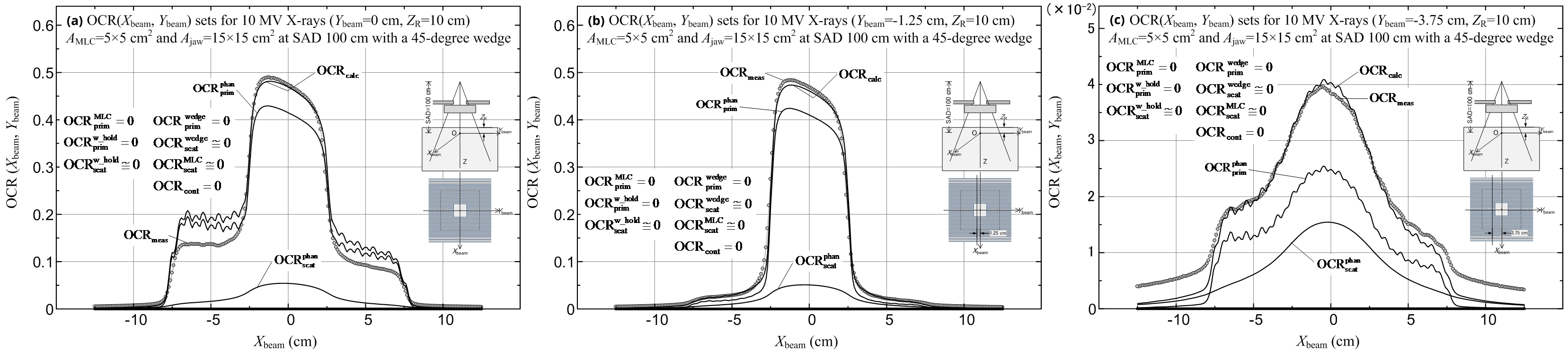
Figures 21a-d show the OCR_calc (including its components) and OCR_meas datasets for Z_R = 2.5 cm with the use of the 60° wedge for a combination of A_MLC = 5 × 5 cm² and A_jaw = 15 × 15 cm² fields: diagram (a) is for Y_beam = 0 cm (details of the lower dose region are shown in diagram (b)); diagram (c) is for Y_beam = -1.25 cm; and diagram (d) is for Y_beam = -3.75 cm. Almost the same calculation accuracy was also observed for the other OCR datasets. It should be noted that the dose leakage characteristics of the MLC are almost the same as those obtained by using a Monte Carlo simulation model [25] (Figures 20a, c and Figures 21a, d).

Figure 21 Graphs of the OCR_calc (including its components) and OCR_meas (in points) datasets, with the X_beam value varied and (a) Y_beam = 0 cm (details of the lower dose region are shown in (b)), (c) Y_beam = -1.25 cm, and (d) Y_beam = -3.75 cm on the isocenter plane at a reference depth of Z_R = 2.5 cm, with the use of a 60° wedge in the direction of the X_beam axis for A_MLC = 5 × 5 cm² and A_jaw = 15 × 15 cm². 10-MV X-rays, SAD = 100 cm (each reference dose was obtained at Z_R = 2.5 cm using the open A_jaw field).

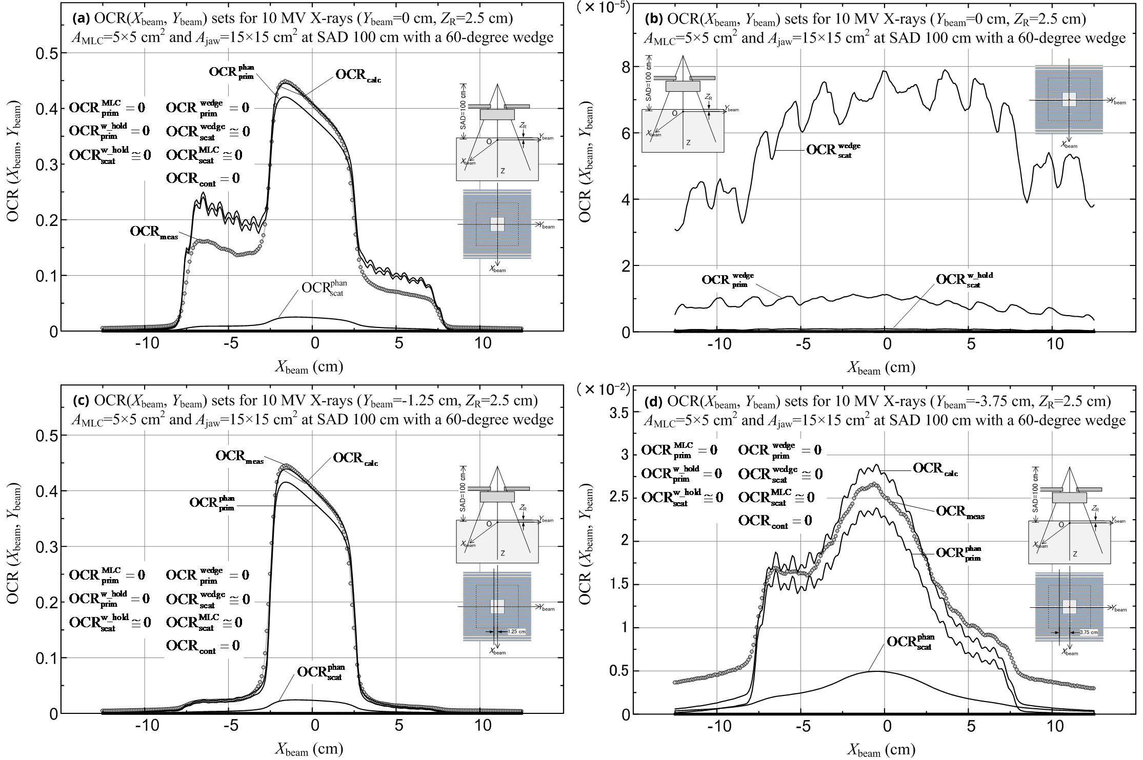
As the above-described PDD and OCR datasets show, the OCR datasets can, in general, reflect levels of dose calculation accuracy to a greater extent than the PDD datasets can. One of the most basic functions for a given linear accelerator is the OCR_source function, defined in an open infinite A_jaw field (equation 23). As the OCR_source function used in this study shows, it may not be reasonable to assume that the OCR_source function is determined only by the off-axis distance on the isocenter plane; instead, it should generally be determined by the 2D position of (X₀, Y₀). Moreover, the magnitude of ρ_{wedge_factor} for each wedge should be determined after acquisition of an accurate OCR_source dataset.

We performed theoretical and experimental studies on 10-MV X-ray dose calculations in water phantoms with multileaf collimation (MLC) and/or wedge filtration using a linear accelerator equipped with (in order from the source side) a pair of upper jaws, a pair of lower jaws, an MLC and a wedge filter. The dose calculation simulations were performed, focusing on percentage depth dose (PDD) and off-center ratio (OCR) datasets.

The dose calculations were based on a convolution method using primary and scatter dose kernels formed for energy bins of X-ray spectra reconstructed as a function of the off-axis distance. We used the MLC leaf-field output subtraction method to calculate the in-air beam intensity for points on the isocenter plane for an open MLC field under a given jaw field, employing a small, extended radiation source on the X-ray target and a large, extended radiation source on the flattening filter. The in-air beam intensity was then decomposed into each energy-bin component (E_N) of the reconstructed X-ray spectra.

The 3D structures of the jaw collimator, MLC and wedge devices were replaced with 2D plates for simple dose calculation. The in-phantom dose calculation was performed by treating the phantom, the wedge, and the MLC as parts of a unified irradiated body, where we proposed to use a factor of μ_med(E_N) ⁄ μ_water(E_N) (the relative attenuation factor) for each energy-bin component (E_N), instead of the relative electron density (ρ_e), for the medium of each volume element within the unified irradiated body, where μ_med(E_N) and μ_water(E_N) are the linear attenuation coefficients for E_N photons of the volume element material and water.